Next, you will learn about code chunks in R Markdown files.

You have already learned that an .Rmd document contains three parts

1. A YAML header.
2. Text chunks in markdown syntax that describe your processing workflow or are the text for your report.
3. Code chunks that process, visualize and/or analyze your data.

Let’s break down code chunks in .Rmd files.

Data Tip: You can add code output or an R object name to markdown segments of an RMD. For more, view this R Markdown documentation.

Code Chunks

Code chunks in an R Markdown document contain your R code. All code chunks start and end with ``` – three backticks or graves. On your keyboard, the backticks can be found on the same key as the tilde (~). Graves are not the same as an apostrophe!

A code chunk looks like this:

```{r chunk-name-with-no-spaces}
# code goes here
 ```

The first line: ```{r chunk-name-with-no-spaces} contains the language (r) in this case, and the name of the chunk. Specifying the language is mandatory. Next to the {r}, there is a chunk name. The chunk name is not necessarily required however, it is good practice to give each chunk a unique name to support more advanced knitting approaches.

Optional challenge: Add code chunks to your R Markdown file

Continue to add to the .Rmd document that you created in the previous lesson. Below the last section that you’ve just added, create a code chunk that performs some basic math.

```{r perform-math }
# perform addition
a <- 1+2

b <- 234

# subtract a from b
final_answer <- b - a

# write out the final answer variable
final_answer

```

Then, add another chunk. Give it a different name.

```{r math-part-two }

   # More math!
   a * b

   a * b / final_answer

 ```

Now run the code in this chunk.

You can run code chunks:

• Line-by-line: With cursor on current line, Ctrl + Enter (Windows/Linux) or Command + Enter (Mac OS X).
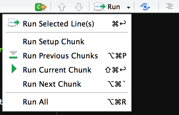
• By chunk: You can run the entire chunk (or multiple chunks) by clicking on the Chunks dropdown button in the upper right corner of the script environment and choosing the appropriate option. Keyboard shortcuts are available for these options.

Comment Your Code

Notice that in each of your code chunks, you’ve introduced comments. Comments are lines in our code that are not run by R. However they allow us to describe the intent of our code. Get in the habit of adding comments as you code. You will learn more about this when you break down scientific programming in R in a later tutorial.

Code Chunk Options

You can add options to each code chunk. These options allow you to customize how or if you want code to be processed or appear on the rendered output (pdf document, html document, etc). Code chunk options are added on the first line of a code chunk after the name, within the curly brackets.

The example below, is a code chunk that will not be “run”, or evaluated, by R. The code within the chunk will appear on the output document, however there will be no outputs from the code.

```{r intro-option, eval = FALSE}
# this is a comment. text, next to a comment, is not processed by R
# comments will appear on your rendered r markdown document
1+2
 ```

One example of using eval = FALSE is for a code chunk that exports a file such as a figure graphic or a text file. You may want to show or document the code that you used to export that graphic in your html or pdf document, but you don’t need to actually export that file each time you create a revised html or pdf document.

3 Common Chunk Options: Eval, Echo & Results

Three common code chunk options are:

• eval = FALSE: Do not evaluate (or run) this code chunk when knitting the RMD document. The code in this chunk will still render in our knitted html output, however it will not be evaluated or run by R.
• echo=FALSE: Hide the code in the output. The code is evaluated when the Rmd file is knit, however only the output is rendered on the output document.
• results=hide: The code chunk will be evaluated but the results or the code will not be rendered on the output document. This is useful if you are viewing the structure of a large object (e.g. outputs of a large data.frame which is the equivalent of a spreadsheet in R).

Multiple code chunk options can be used for the same chunk.

```{r testing-arguments, eval = FALSE }

   # More math!
   a * b

   a * b / final_answer

 ```

```{r testing-arguments, echo=FALSE }

    # More math!
    a * b

    a * b / final_answer

  ```

```{r testing-arguments, results="hide" }

     # More math!
     a * b

     a * b / final_answer

   ```

You will knit your R Markdown document to .html in the next lesson.