Lesson 1. Add a Basemap to an R Markdown Report Using ggmap
Basemaps in R - Earth analytics course module
Welcome to the first lesson in the Basemaps in R module. This module covers using ggmap to create basemaps in r / rmarkdown and how to overlay raster data on top of a hillshade.Learning Objectives
After completing this tutorial, you will be able to:
- Create a quick basemap using
ggmapOR - Create a quick basemap using the
mapspackage.
What You Need
You need R and RStudio to complete this tutorial. Also you should have an earth-analytics directory set up on your computer with a /data directory with it.
- install devtools:
install.packages('devtools') - install ggmap from github:
devtools::install_github("dkahle/ggmap") install maps:
install.packages('maps')- How to set up R / RStudio
- Set up your working directory
# install devtools
#install.packages("devtools")
# install ggmap from dev space
# devtools::install_github("dkahle/ggmap")

library(ggmap)
Create Basemap
First, create a basemap that shows the location of the stream gage in Boulder, Colorado.
myMap <- get_stamenmap(bbox = c(left = -105.4969,
                                    bottom = 39.8995,
                                    right = -104.9579,
                                    top = 40.1274),
          maptype = "terrain",
          crop = FALSE,
          zoom = 6)
# plot map
ggmap(myMap)
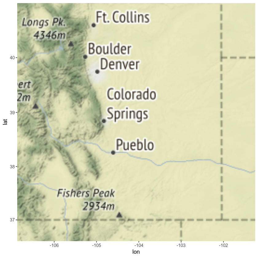
There are many other basemap options. Check out the help for get_stamenmap by typing ??get_stamenmap into the R console.
Let’s check out the stamen watercolor maps. Notice that I zoomed out some here so you can see the full effect of the new basemap.
myMap <- get_stamenmap(bbox = c(left = -105.4969,
                                    bottom = 39.8995,
                                    right = -104.9579,
                                    top = 40.1274),
          maptype = "watercolor",
          crop = FALSE,
          zoom = 4)
# plot map
ggmap(myMap)
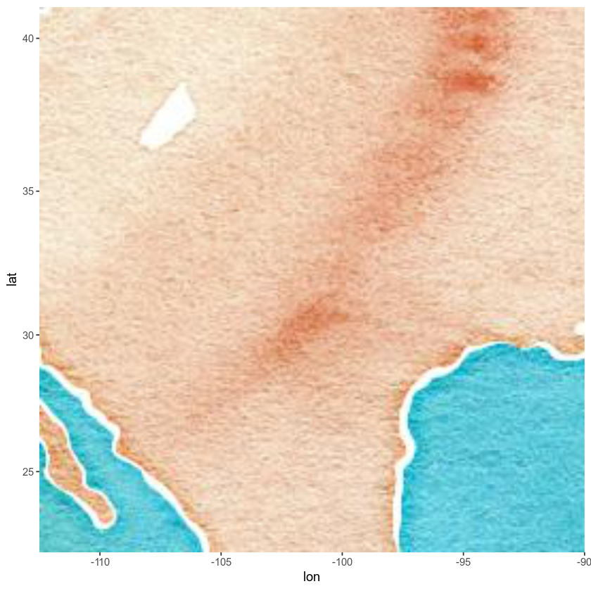
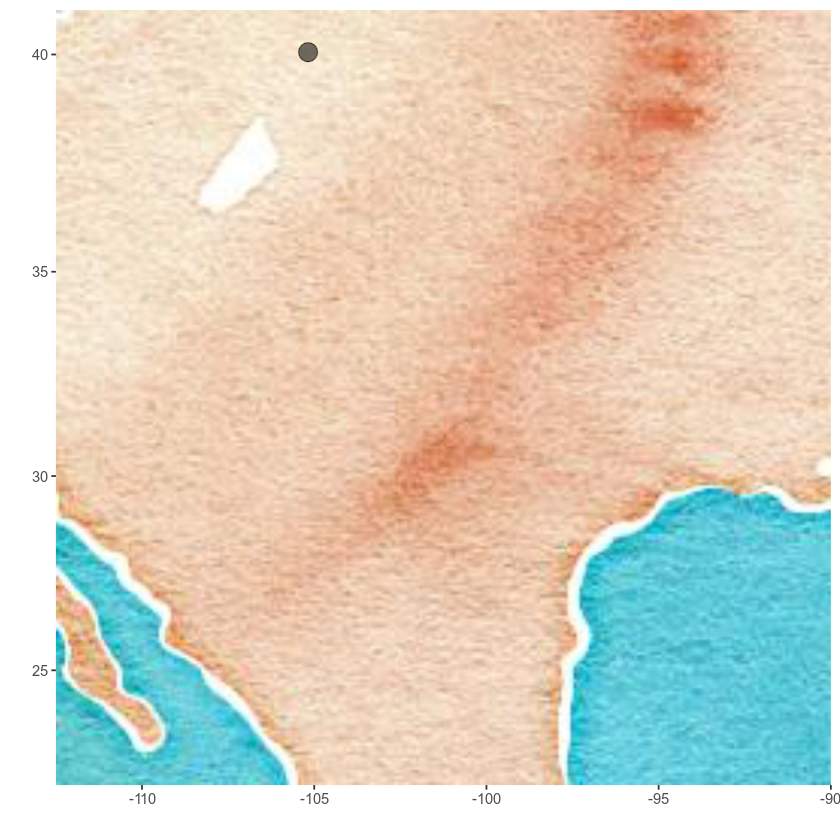
Ok, enough of the map play time - let’s get back to business. Next, let’s add a point to your map representing the location of your actual stream gage data.
Latitude: 40.051667 Longitude: 105.178333
USGS gage 06730200 40°03’06” 105°10’42”
# add points to your map
# creating a sample data.frame with your lat/lon points
gage_location <- data.frame(lon = c(-105.178333), lat = c(40.051667))

# create a map with a point location for boulder.
ggmap(myMap) + labs(x = "", y = "") +
  geom_point(data = gage_location, aes(x = lon, y = lat, fill = "red", alpha = 0.2), size = 5, shape = 19) +
  guides(fill = FALSE, alpha = FALSE, size = FALSE)
Alternative - Maps Package
If you can’t install ggmap, you can also create nice basemaps using the maps package. The maps package allows you to quickly create basemaps of study areas. It utilizes a set of vector based layers including layers that map:
- countries across the globe
- the United States and associated counties
- and more
You can use the maps package, combined with the R base plot functions to add base layers to your map.
#install.packages('maps')
library(maps)
library(mapdata)
Create a Basic Map of the United States
map('state')
# add a title to your map
title('Map of the United States')
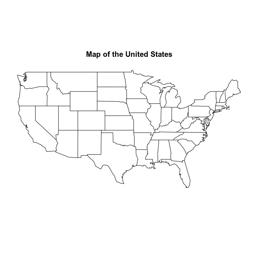
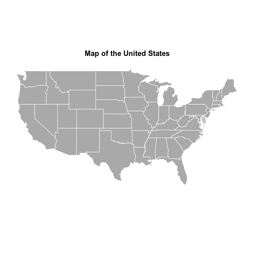
Plot using basemap - customize colors.
map('state', col = "darkgray",
    fill = TRUE,
    border = "white")
# add a title to your map
title('Map of the United States')
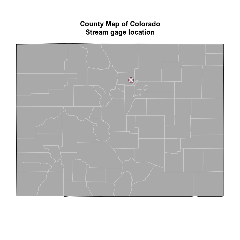
Create a map of Colorado with county boundaries.
map('county', regions = "Colorado", col = "darkgray", fill = TRUE, border = "grey80")
map('state', regions = "Colorado", col = "black", add = TRUE)
# add the x, y location of the stream guage using the points
# notice i used two colors adn sized to may the symbol look a little brighter
points(x = -105.178333, y = 40.051667, pch = 21, col = "violetred4", cex = 2)
points(x = -105.178333, y = 40.051667, pch = 8, col = "white", cex = 1.3)
# add a title to your map
title('County Map of Colorado\nStream gage location')
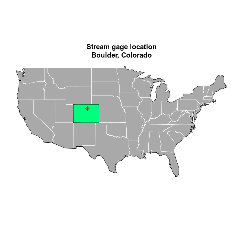
You can stack several map layers using add = TRUE. Notice you can create multi-line titles using \n.
map('state', fill = TRUE, col = "darkgray", border = "white", lwd = 1)
map(database = "usa", lwd = 1, add = TRUE)
# add the adjacent parts of the US; can't forget my homeland
map("state", "colorado", col = "springgreen",
    lwd = 1, fill = TRUE, add = TRUE)
# add gage location
title("Stream gage location\nBoulder, Colorado")
# add the x, y location of hte stream guage using the points
points(x = -105.178333, y = 40.051667, pch = 8, col = "red", cex = 1.3)
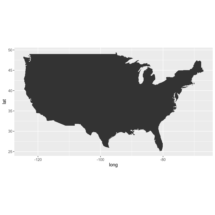
Or you can plot with ggplot
usa <- map_data("usa")
head(usa)
##        long      lat group order region subregion
## 1 -101.4078 29.74224     1     1   main      <NA>
## 2 -101.3906 29.74224     1     2   main      <NA>
## 3 -101.3620 29.65056     1     3   main      <NA>
## 4 -101.3505 29.63911     1     4   main      <NA>
## 5 -101.3219 29.63338     1     5   main      <NA>
## 6 -101.3047 29.64484     1     6   main      <NA>
plot with ggplot.
ggplot() +
  geom_polygon(data = usa, aes(x = long, y = lat, group = group)) +
  coord_fixed(1.3)
Share on
Twitter Facebook Google+ LinkedIn
Leave a Comment