About Vector Data

Vector data are composed of discrete geometric locations (x,y values) known as vertices that define the “shape” of the spatial object. The organization of the vertices determines the type of vector that you are working with: point, line or polygon.

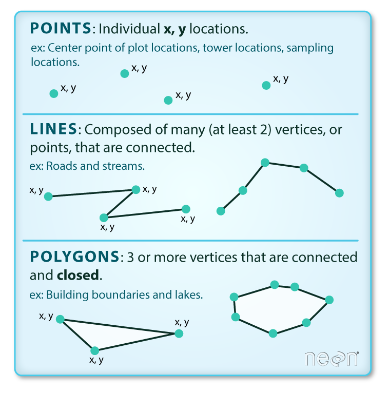
• Points: Each individual point is defined by a single x, y coordinate. There can be many points in a vector point file. Examples of point data include: sampling locations, the location of individual trees or the location of plots.
• Lines: Lines are composed of many (at least 2) vertices, or points, that are connected. For instance, a road or a stream may be represented by a line. This line is composed of a series of segments, each “bend” in the road or stream represents a vertex that has defined x, y location.
• Polygons: A polygon consists of 3 or more vertices that are connected and “closed”. Thus the outlines of plot boundaries, lakes, oceans, and states or countries are often represented by polygons. Occasionally, a polygon can have a hole in the middle of it (like a doughnut), this is something to be aware of but not an issue you will deal with in this tutorial.

Data Tip: Sometimes boundary layers such as states and countries, are stored as lines rather than polygons. However, these boundaries, when represented as a line, will not create a closed object with a defined “area” that can be “filled”.

Shapefiles: Points, Lines, and Polygons

Geospatial data in vector format are often stored in a shapefile format. Because the structure of points, lines, and polygons are different, each individual shapefile can only contain one vector type (all points, all lines or all polygons). You will not find a mixture of point, line and polygon objects in a single shapefile.

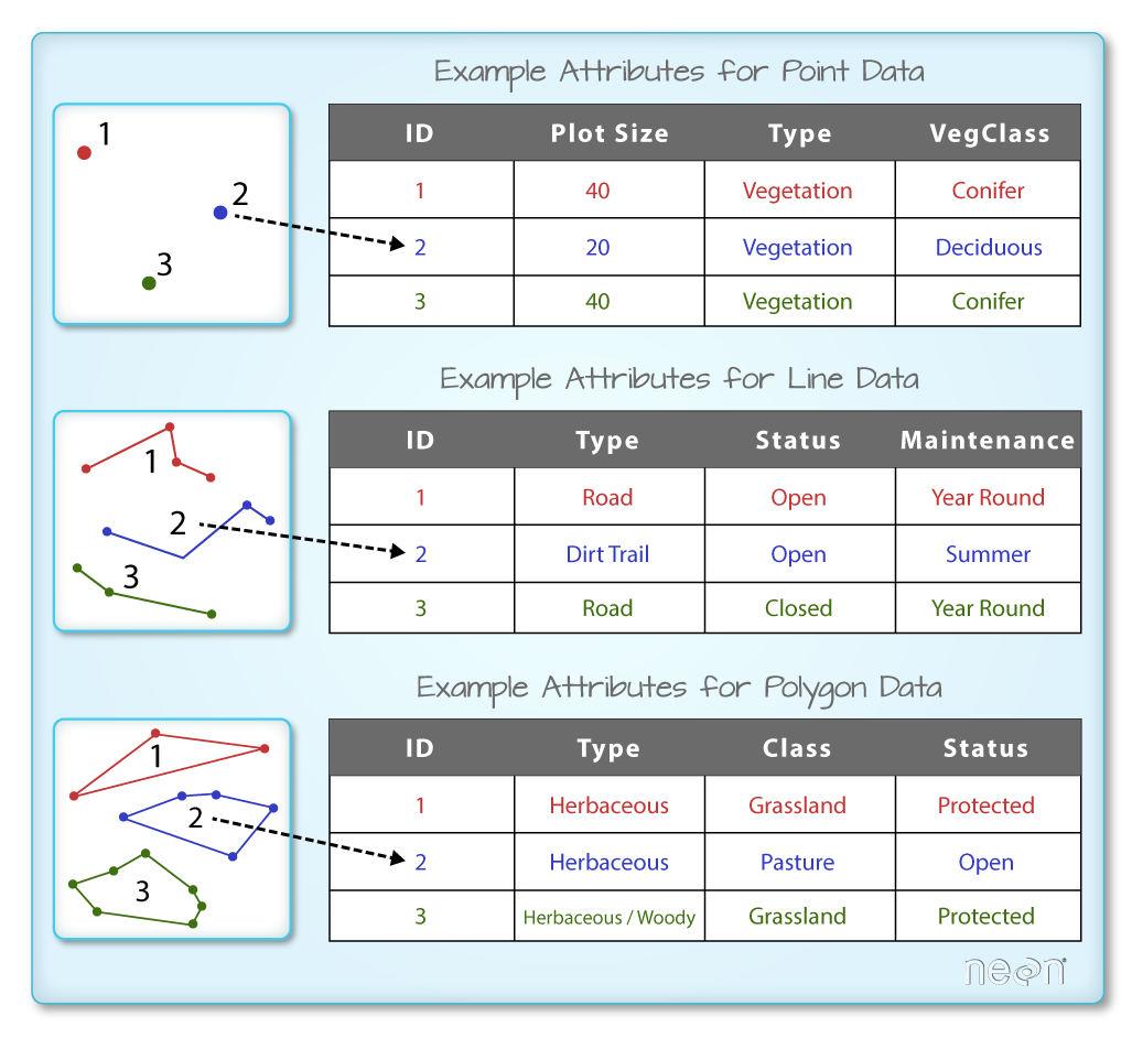
Objects stored in a shapefile often have a set of associated attributes that describe the data. For example, a line shapefile that contains the locations of streams, might contain the associated stream name, stream “order” and other information about each stream line object.

• More about shapefiles can found on Wikipedia.

Import Shapefiles

You will use the rgdal package to work with vector data in R. Notice that the sp package automatically loads when rgdal is loaded. You will also load the raster package so you can explore raster and vector spatial metadata using similar commands.

# work with spatial data; sp package will load with rgdal.
library(rgdal)
library(rgeos)
# for metadata/attributes- vectors or rasters
library(raster)

# set working directory to earth-analytics dir
# setwd("pathToDirHere")

The shapefiles that you will import are:

• A polygon shapefile representing your field site boundary.
• A line shapefile representing roads.
• A point shapefile representing the location of field sites located at the San Joachin field site.

The first shapefile that you will open contains the point locations where trees have been measured at the study site. The data are stored in shapefile format. To import shapefiles you use the R function readOGR().

readOGR() requires two components:

1. The directory where your shapefile lives: data/week-04/california/SJER/vector_data/.
2. The name of the shapefile (without the extension): SJER_plot_centroids.

You can call each element separately

readOGR("path","fileName")

Or you can simply include the entire path to the shp file in the path argument. Both ways to open a shapefile are demonstrated below:

# Import a polygon shapefile: readOGR("path","fileName")
sjer_plot_locations <- readOGR(dsn = "data/week-04/california/SJER/vector_data",
                               "SJER_plot_centroids")
## OGR data source with driver: ESRI Shapefile 
## Source: "/root/earth-analytics/data/week-04/california/SJER/vector_data", layer: "SJER_plot_centroids"
## with 18 features
## It has 5 fields

Data Tip: The acronym, OGR, refers to the OpenGIS Simple Features Reference Implementation. Learn more about OGR.

Shapefile Metadata & Attributes

When you import the SJER_plot_centroids shapefile layer into R the readOGR() function automatically stores information about the data. You are particularly interested in the geospatial metadata, describing the format, CRS, extent, and other components of the vector data, and the attributes which describe properties associated with each individual vector object.

Spatial Metadata

Key metadata for all shapefiles include:

1. Object Type: the class of the imported object.
2. Coordinate Reference System (CRS): the projection of the data.
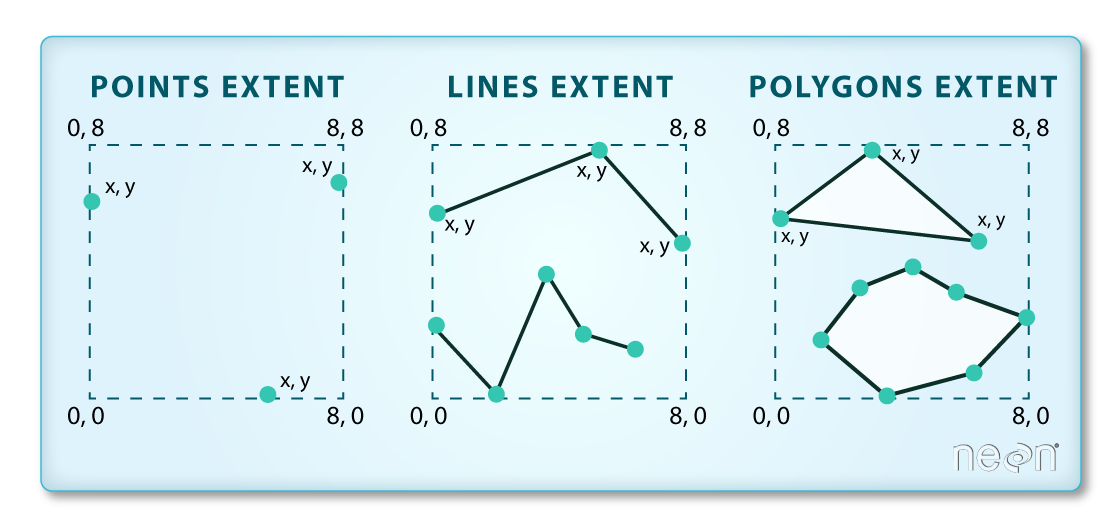
3. Extent: the spatial extent (geographic area that the shapefile covers) of the shapefile. Note that the spatial extent for a shapefile represents the extent for ALL spatial objects in the shapefile.

You can view shapefile metadata using the class, crs and extent methods:

# view just the class for the shapefile
class(sjer_plot_locations)
## [1] "SpatialPointsDataFrame"
## attr(,"package")
## [1] "sp"

# view just the crs for the shapefile
crs(sjer_plot_locations)
## CRS arguments:
##  +proj=utm +zone=11 +datum=WGS84 +units=m +no_defs +ellps=WGS84
## +towgs84=0,0,0

# view just the extent for the shapefile
extent(sjer_plot_locations)
## class      : Extent 
## xmin       : 254738.6 
## xmax       : 258497.1 
## ymin       : 4107527 
## ymax       : 4112168

# view all metadata at same time
sjer_plot_locations
## class       : SpatialPointsDataFrame 
## features    : 18 
## extent      : 254738.6, 258497.1, 4107527, 4112168  (xmin, xmax, ymin, ymax)
## crs         : +proj=utm +zone=11 +datum=WGS84 +units=m +no_defs +ellps=WGS84 +towgs84=0,0,0 
## variables   : 5
## names       :  Plot_ID,  Point,    northing,    easting, plot_type 
## min values  : SJER1068, center, 4107527.074, 254738.618,     grass 
## max values  :  SJER952, center, 4112167.778, 258497.102,     trees

Your sjer_plot_locations object is a polygon of class SpatialPointsDataFrame, in the CRS UTM zone 18N. The CRS is critical to interpreting the object extent values as it specifies units.

Spatial Data Attributes

Each object in a shapefile has one or more attributes associated with it. Shapefile attributes are similar to fields or columns in a spreadsheet. Each row in the spreadsheet has a set of columns associated with it that describe the row element. In the case of a shapefile, each row represents a spatial object - for example, a road, represented as a line in a line shapefile, will have one “row” of attributes associated with it. These attributes can include different types of information that describe objects stored within a shapefile. Thus, your road, may have a name, length, number of lanes, speed limit, type of road and other attributes stored with it.

You view the attributes of a SpatialPointsDataFrame using objectName@data (e.g., sjer_plot_locations@data).

# alternate way to view attributes
sjer_plot_locations@data
##     Plot_ID  Point northing  easting plot_type
## 1  SJER1068 center  4111568 255852.4     trees
## 2   SJER112 center  4111299 257407.0     trees
## 3   SJER116 center  4110820 256838.8     grass
## 4   SJER117 center  4108752 256176.9     trees
## 5   SJER120 center  4110476 255968.4     grass
## 6   SJER128 center  4111389 257078.9     trees
## 7   SJER192 center  4111071 256683.4     grass
## 8   SJER272 center  4112168 256717.5     trees
## 9  SJER2796 center  4111534 256034.4      soil
## 10 SJER3239 center  4109857 258497.1      soil
## 11   SJER36 center  4110162 258277.8     trees
## 12  SJER361 center  4107527 256961.8     grass
## 13   SJER37 center  4107579 256148.2     trees
## 14    SJER4 center  4109767 257228.3     trees
## 15    SJER8 center  4110249 254738.6     trees
## 16  SJER824 center  4110048 256185.6      soil
## 17  SJER916 center  4109617 257460.5      soil
## 18  SJER952 center  4110759 255871.2     grass

In this case, your polygon object only has one attribute: id.

Metadata & Attribute Summary

You can view a metadata & attribute summary of each shapefile by entering the name of the R object in the console. Note that the metadata output includes the class, the number of features, the extent, and the coordinate reference system (crs) of the R object. The last two lines of summary show a preview of the R object attributes.

# view a summary of metadata & attributes associated with the spatial object
summary(sjer_plot_locations)
##                 Length                  Class                   Mode 
##                     18 SpatialPointsDataFrame                     S4

Plot a Shapefile

Next, let’s visualize the data in your R spatialpointsdataframe object using plot().

# create a plot of the shapefile
# 'pch' sets the symbol
# 'col' sets point symbol color
plot(sjer_plot_locations, col = "blue",
     pch = 8)
title("SJER Plot Locations\nMadera County, CA")

Plot Multiple Shapefiles

The plot() function can be used to plot spatial objects. Use the following arguments to add a title to your plot and to layer several spatial objects on top of each other in your plot.

• add = TRUE: overlay a shapefile or raster on top the existing plot. This argument mimics layers in a typical GIS application like QGIS.
• main = "": add a title to the plot. To add a line break to your title, use \n where the line break should occur.

# Plot multiple shapefiles
plot(sjer_crop_extent, col = "lightgreen", main ="NEON SJER Field Site")

# Use the pch element to adjust the symbology of the points
plot(sjer_plot_locations,
  add  = TRUE,
  pch = 19,
  col = "purple")