Lesson 2. Use Raster Data for Earth Data Science
Fundamentals of Raster Data in Python
In this lesson, you will learn fundamental concepts related to working with raster data in Python, including understanding the spatial attributes of raster data, how to open raster data, and how to visually plot the data.
Learning Objectives
After completing this lesson, you will be able to:
- Open raster data using Rioxarray in Python.
- Be able to plot spatial raster data using EarthPy in Python.
Suggested Readings
Before starting this lesson, read the What is a Raster section of this page of the Earth Lab website to familiarize yourself with the concept of raster data.
What is Raster data?
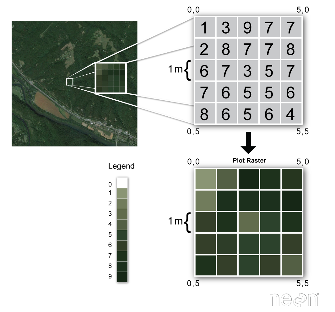
Raster or “gridded” data are stored as a grid of values which are rendered on a map as pixels. Each pixel value represents an area on the Earth’s surface making the data spatial. A raster file is composed of regular grid of cells, all of which are the same size. You’ve looked at and used rasters before if you’ve looked at photographs or imagery in a tool like Google Earth. However, the raster files that you will work with are different from photographs in that they are spatially referenced. Each pixel represents an area of land on the ground. That area is defined by the spatial resolution of the raster.
Data Tip: For more information on rasters, how they work, and the types of data stored in rasters, see this chapter on using raster data from the earth data science intermediate textbook.
Raster Data Can Have One or More Layers
Raster data can have one or more layers. An elevation model for example will often just have one layer representing the elevation of the earth’s surface for a particular location. However, other data including images and time series data, may result in a raster file that is composed of multiple layers. Different file types can be used to accomodate different sizes and structures of raster data.
There Are Many Different File Raster File Formats
There are many different file types that are used to store raster data.
Raster Data Stored As Single Files
Some datasets such as landsat and NAIP are stored in single files. For landsat, often you will find each band stored as a separate .tif file. NAIP stores all bands in on .tif file. Common file types for raster data stored as a single file include:
- .tif / .tiff: Stands for Tagged Image File Format. One of the most common ways to store raster data. How some image satellites, such as Landsat, share their data.
- .asc: Stands for ASCII Raster Files. This is a text based format that stores raster data. This format is used given it’s simple to store and distribute.
Hierarchical Data Formats
Hierarchical data formats can store many different types of data in one single file. These formats are optimal for larger data sets where you may want to subset or only work with parts of the data at one time. Hierarchical data can be a bit more involved to work with but they tend to make processing more efficient. Common file types for this data storage method include:
- .hdf / .hdf5: Stands for Hierarchical Data Format. One of the most common hierarchical was to store raster data. How some image satellites, such as MODIS, share their data.
- .nc (NetCDF): Stands for Network Common Data Form. A common way to store climate data.
Data Tip: Learn more about working with GeoTiff files in this earth data science textbook lesson.. Learn more about working with HDF4 files (the format used to store MODIS data) in this earth data science textbook chapter.
What Types of Data Are Stored In Rasters?
Some examples of data that often are provided in a raster format include:
- Satellite imagery
- Land use over large areas
- Elevation data
- Weather data
- Bathymetry data
Next you will open and work with some raster data. To begin setup your notebook with the required python packages.
# Import necessary packages
import os

import matplotlib.pyplot as plt
import numpy as np
import geopandas as gpd
import rioxarray as rxr

# Earthpy is an earthlab package to work with spatial data
import earthpy as et
import earthpy.plot as ep

# Get data and set working directory
et.data.get_data("colorado-flood")
os.chdir(os.path.join(et.io.HOME, 'earth-analytics', 'data'))
Downloading from https://ndownloader.figshare.com/files/16371473
Extracted output to /root/earth-analytics/data/colorado-flood/.
Open Raster Data in Open Source Python Using Rioxarray
You can open raster data in Python using rioxarray. The code below can be used to open up a raster file:
# Read the data in and call it lidar_dtm (this is the variable name)
lidar_dtm = rxr.open_rasterio(lidar_dem_path, masked=True)
The code does the following:
rxr.open_rasterio- rxr is the alias for rioxarray. At the top of your code you include rioxarray:import rioxarray as rxr.masked=Truestatement will mask allnodatavalues in your array. This means that they will not be plotted and also that they will not be included in math calculations inPython.
The data that you will work with below - filename: pre_DTM.tif is lidar (Light Detection and Ranging) derived elevation data. The file format is a .tif file. The data represent a Digital Terrain Model (DTM). You can learn more about DTMs in this earth data science lesson on lidar data.
Below, you create a path to the file you want to open.
# Create a path to file
lidar_dtm_path = os.path.join("colorado-flood",
                              "spatial",
                              "boulder-leehill-rd",
                              "pre-flood",
                              "lidar",
                              "pre_DTM.tif")
lidar_dtm_path
'colorado-flood/spatial/boulder-leehill-rd/pre-flood/lidar/pre_DTM.tif'
Next, open up your data.
# Open and read in the digital terrain model
# Note that rxr is the alias for rioxarray
lidar_dtm = rxr.open_rasterio(lidar_dtm_path, masked=True)

# View the data - notice the data structure is different from geopandas data
# which you explored in the last lesson
lidar_dtm
<xarray.DataArray (band: 1, y: 2000, x: 4000)>
[8000000 values with dtype=float64]
Coordinates:
  * band         (band) int64 1
  * y            (y) float64 4.436e+06 4.436e+06 ... 4.434e+06 4.434e+06
  * x            (x) float64 4.72e+05 4.72e+05 4.72e+05 ... 4.76e+05 4.76e+05
    spatial_ref  int64 0
Attributes:
    scale_factor:  1.0
    add_offset:    0.0
grid_mapping: spatial_ref- band: 1
- y: 2000
- x: 4000
- ...
[8000000 values with dtype=float64]
- band(band)int641
array([1])
- y(y)float644.436e+06 4.436e+06 ... 4.434e+06
array([4435999.5, 4435998.5, 4435997.5, ..., 4434002.5, 4434001.5, 4434000.5])
- x(x)float644.72e+05 4.72e+05 ... 4.76e+05
array([472000.5, 472001.5, 472002.5, ..., 475997.5, 475998.5, 475999.5])
- spatial_ref()int640
- crs_wkt :
- PROJCS["WGS 84 / UTM zone 13N",GEOGCS["WGS 84",DATUM["WGS_1984",SPHEROID["WGS 84",6378137,298.257223563,AUTHORITY["EPSG","7030"]],AUTHORITY["EPSG","6326"]],PRIMEM["Greenwich",0,AUTHORITY["EPSG","8901"]],UNIT["degree",0.0174532925199433,AUTHORITY["EPSG","9122"]],AUTHORITY["EPSG","4326"]],PROJECTION["Transverse_Mercator"],PARAMETER["latitude_of_origin",0],PARAMETER["central_meridian",-105],PARAMETER["scale_factor",0.9996],PARAMETER["false_easting",500000],PARAMETER["false_northing",0],UNIT["metre",1,AUTHORITY["EPSG","9001"]],AXIS["Easting",EAST],AXIS["Northing",NORTH],AUTHORITY["EPSG","32613"]]
- semi_major_axis :
- 6378137.0
- semi_minor_axis :
- 6356752.314245179
- inverse_flattening :
- 298.257223563
- reference_ellipsoid_name :
- WGS 84
- longitude_of_prime_meridian :
- 0.0
- prime_meridian_name :
- Greenwich
- geographic_crs_name :
- WGS 84
- horizontal_datum_name :
- World Geodetic System 1984
- projected_crs_name :
- WGS 84 / UTM zone 13N
- grid_mapping_name :
- transverse_mercator
- latitude_of_projection_origin :
- 0.0
- longitude_of_central_meridian :
- -105.0
- false_easting :
- 500000.0
- false_northing :
- 0.0
- scale_factor_at_central_meridian :
- 0.9996
- spatial_ref :
- PROJCS["WGS 84 / UTM zone 13N",GEOGCS["WGS 84",DATUM["WGS_1984",SPHEROID["WGS 84",6378137,298.257223563,AUTHORITY["EPSG","7030"]],AUTHORITY["EPSG","6326"]],PRIMEM["Greenwich",0,AUTHORITY["EPSG","8901"]],UNIT["degree",0.0174532925199433,AUTHORITY["EPSG","9122"]],AUTHORITY["EPSG","4326"]],PROJECTION["Transverse_Mercator"],PARAMETER["latitude_of_origin",0],PARAMETER["central_meridian",-105],PARAMETER["scale_factor",0.9996],PARAMETER["false_easting",500000],PARAMETER["false_northing",0],UNIT["metre",1,AUTHORITY["EPSG","9001"]],AXIS["Easting",EAST],AXIS["Northing",NORTH],AUTHORITY["EPSG","32613"]]
- GeoTransform :
- 472000.0 1.0 0.0 4436000.0 0.0 -1.0
array(0)
- scale_factor :
- 1.0
- add_offset :
- 0.0
- grid_mapping :
- spatial_ref
Explore Raster Data Values & Structure
Next, have a look at the data. Notice that the data structure of type() of Python object returned by rioxarray is an xarray DataArray. This contains metadata about the array, as well as the data for the array stored in a numpy array. Numpy arrays are an efficient way to store and work with raster data in python. You will learn more about working with numpy arrays in the numpy array chapter of the introduction to earth data science textbook
Data Tip: To view the numpy array stored inside of an xarray DataArray, you can access it by putting .values at the end of your Rioxarray variable’s name. For example, rioxarray_name.values will return a numpy array with all the values stored in it. We use .values to plot with the earthpy plot_rgb function, since that needs a numpy array as an input!
type(lidar_dtm)
xarray.core.dataarray.DataArray
# View the min and max values of the array
print(lidar_dtm.min(), lidar_dtm.max())
<xarray.DataArray ()>
array(1676.20996094)
Coordinates:
    spatial_ref  int64 0 <xarray.DataArray ()>
array(2087.42993164)
Coordinates:
    spatial_ref  int64 0
# View the dimensions of the array (rows, columns)
lidar_dtm.shape
(1, 2000, 4000)
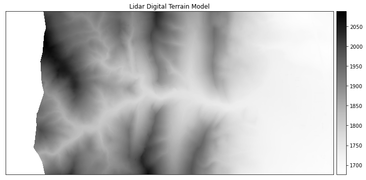
Finally you can plot your data. For plotting you will use earthpy.plot_bands.
ep.plot_bands(lidar_dtm,
              scale=False,
              cmap='Greys',
              title="Lidar Digital Terrain Model")
plt.show()
Challenge 1: Explore Elevation Data Values
Look closely at the plot above. What do you think the colors and numbers represent in the plot?
What units do the numbers represents?
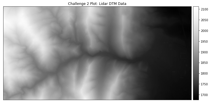
Challenge 2: Open & Plot a Raster Dataset
The above lidar DTM that you opened represents a dataset produced before a flood occurred in 2013 in Colorado. A path to a second lidar dataset which is for the same area but from data collected after the flood is below.
Use the code below to create a path to the post-flood data. Then do the following using the code above as a guide to open and plot your data:
- Use
rioxarrayto open the data as a numpy array following the code that you used above - View the min and max data values for the output numpy array
- Create a plot of the data
# Add the code here to open, show, and close the raster dataset.

lidar_dem_path_post_flood = os.path.join("data", "colorado-flood", "spatial",
                                         "boulder-leehill-rd", "post-flood", "lidar",
                                         "post_DTM.tif")
Hint: Don’t forget to use rxr.open_rasterio() and assign the output to a variable! Also, don’t forget to call .values on your rioxarray when plotting it with plot_rgb, that function needs a numpy array input to work!
An example of what your plot should look like is below.
Imagery - Another Type of Raster Data
Another type of raster data that you may see is imagery. If you have used Google Maps or another mapping tool that has an imagery layer, you are looking at raster data. You can open and plot imagery data using Python as well.
Below you download and open up some NAIP data that were collected before a fire that occured close to Nederland, Colorado.
Data Tip: NAIP data is imagery collected by the United States Department of Agriculture every 2 years across the United States. Learn more about NAIP data in this chapter of the earth data science intermediate textbook.
# Download NAIP data
et.data.get_data(url="https://ndownloader.figshare.com/files/23070791")
Downloading from https://ndownloader.figshare.com/files/23070791
Extracted output to /root/earth-analytics/data/earthpy-downloads/naip-before-after
'/root/earth-analytics/data/earthpy-downloads/naip-before-after'
# Create a path for the data file - notice it is a .tif file
naip_pre_fire_path = os.path.join("earthpy-downloads",
                                  "naip-before-after",
                                  "pre-fire",
                                  "crop",
                                  "m_3910505_nw_13_1_20150919_crop.tif")

naip_pre_fire_path
'earthpy-downloads/naip-before-after/pre-fire/crop/m_3910505_nw_13_1_20150919_crop.tif'
# Open the data using rioxarray
naip_pre_fire = rxr.open_rasterio(naip_pre_fire_path)

naip_pre_fire
<xarray.DataArray (band: 4, y: 2312, x: 4377)>
[40478496 values with dtype=int16]
Coordinates:
  * band         (band) int64 1 2 3 4
  * y            (y) float64 4.427e+06 4.427e+06 ... 4.425e+06 4.425e+06
  * x            (x) float64 4.572e+05 4.572e+05 ... 4.615e+05 4.615e+05
    spatial_ref  int64 0
Attributes:
    STATISTICS_MAXIMUM:  239
    STATISTICS_MEAN:     nan
    STATISTICS_MINIMUM:  32
    STATISTICS_STDDEV:   nan
    _FillValue:          -32768.0
    scale_factor:        1.0
    add_offset:          0.0
grid_mapping: spatial_ref- band: 4
- y: 2312
- x: 4377
- ...
[40478496 values with dtype=int16]
- band(band)int641 2 3 4
array([1, 2, 3, 4])
- y(y)float644.427e+06 4.427e+06 ... 4.425e+06
array([4426951.5, 4426950.5, 4426949.5, ..., 4424642.5, 4424641.5, 4424640.5])
- x(x)float644.572e+05 4.572e+05 ... 4.615e+05
array([457163.5, 457164.5, 457165.5, ..., 461537.5, 461538.5, 461539.5])
- spatial_ref()int640
- crs_wkt :
- PROJCS["UTM Zone 13, Northern Hemisphere",GEOGCS["GRS 1980(IUGG, 1980)",DATUM["unknown",SPHEROID["GRS80",6378137,298.257222101],TOWGS84[0,0,0,0,0,0,0]],PRIMEM["Greenwich",0],UNIT["degree",0.0174532925199433,AUTHORITY["EPSG","9122"]]],PROJECTION["Transverse_Mercator"],PARAMETER["latitude_of_origin",0],PARAMETER["central_meridian",-105],PARAMETER["scale_factor",0.9996],PARAMETER["false_easting",500000],PARAMETER["false_northing",0],UNIT["metre",1,AUTHORITY["EPSG","9001"]],AXIS["Easting",EAST],AXIS["Northing",NORTH]]
- semi_major_axis :
- 6378137.0
- semi_minor_axis :
- 6356752.314140356
- inverse_flattening :
- 298.257222101
- reference_ellipsoid_name :
- GRS80
- longitude_of_prime_meridian :
- 0.0
- prime_meridian_name :
- Greenwich
- geographic_crs_name :
- GRS 1980(IUGG, 1980)
- horizontal_datum_name :
- unknown
- projected_crs_name :
- UTM Zone 13, Northern Hemisphere
- grid_mapping_name :
- transverse_mercator
- latitude_of_projection_origin :
- 0.0
- longitude_of_central_meridian :
- -105.0
- false_easting :
- 500000.0
- false_northing :
- 0.0
- scale_factor_at_central_meridian :
- 0.9996
- towgs84 :
- [0.0, 0.0, 0.0, 0.0, 0.0, 0.0, 0.0]
- spatial_ref :
- PROJCS["UTM Zone 13, Northern Hemisphere",GEOGCS["GRS 1980(IUGG, 1980)",DATUM["unknown",SPHEROID["GRS80",6378137,298.257222101],TOWGS84[0,0,0,0,0,0,0]],PRIMEM["Greenwich",0],UNIT["degree",0.0174532925199433,AUTHORITY["EPSG","9122"]]],PROJECTION["Transverse_Mercator"],PARAMETER["latitude_of_origin",0],PARAMETER["central_meridian",-105],PARAMETER["scale_factor",0.9996],PARAMETER["false_easting",500000],PARAMETER["false_northing",0],UNIT["metre",1,AUTHORITY["EPSG","9001"]],AXIS["Easting",EAST],AXIS["Northing",NORTH]]
- GeoTransform :
- 457163.0 1.0 0.0 4426952.0 0.0 -1.0
array(0)
- STATISTICS_MAXIMUM :
- 239
- STATISTICS_MEAN :
- nan
- STATISTICS_MINIMUM :
- 32
- STATISTICS_STDDEV :
- nan
- _FillValue :
- -32768.0
- scale_factor :
- 1.0
- add_offset :
- 0.0
- grid_mapping :
- spatial_ref
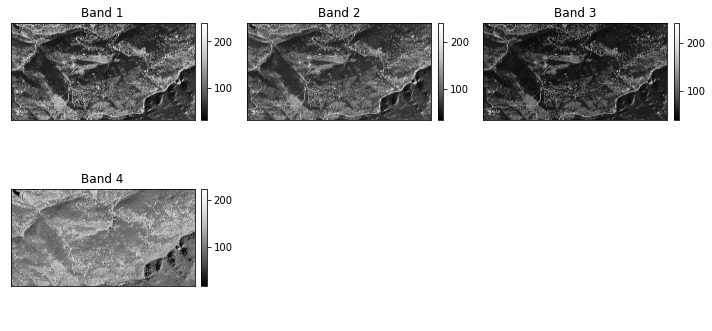
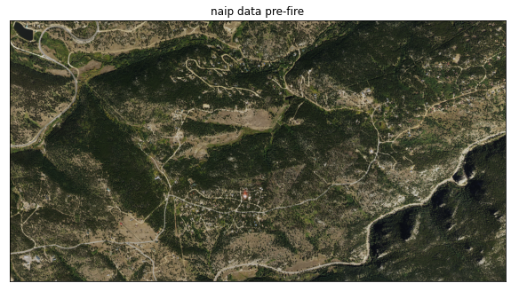
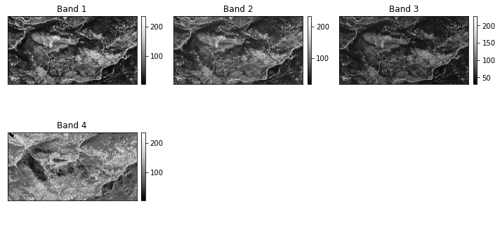
Plotting imagery is a bit different because imagery is composed of multiple bands. While we won’t get into the specifics of bands and images in this lesson, you can see below that an image is composed of multiple layers of information.
You can plot each band individually as you see below using plot_bands(). Or you can plot a color image, similar to the image that your camera stores when you take a picture.
# Plot each layer or band of the image separately
ep.plot_bands(naip_pre_fire, figsize=(10, 5))
plt.show()
# Plot color image
#
ep.plot_rgb(naip_pre_fire.values,
            title="naip data pre-fire")
plt.show()
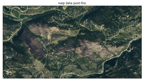
Challenge: Plot NAIP Imagery Post Fire
In the code below, you see a path to a NAIP dataset that was collected after the fire in Colorado. Use that path to:
- Open the post fire data
- Plot a color version of data using
plot_rgb()
# Add the code here to open the raster and read the numpy array inside it
# Create a path for the data file - notice it is a .tif file
naip_post_fire_path = os.path.join("earthpy-downloads",
                                   "naip-before-after",
                                   "post-fire",
                                   "crop",
                                   "m_3910505_nw_13_1_20170902_crop.tif")

naip_post_fire_path
'earthpy-downloads/naip-before-after/post-fire/crop/m_3910505_nw_13_1_20170902_crop.tif'


Share on
Twitter Facebook Google+ LinkedIn
Leave a Comment