Lesson 1. Intro to Pandas Dataframes
Work with Scientific Data Using Pandas Dataframes - Intro to earth data science textbook course module
Welcome to the first lesson in the Work with Scientific Data Using Pandas Dataframes module. Pandas dataframes are a commonly used scientific data structure in Python that store tabular data using rows and columns with headers. Learn how to import data into pandas dataframes and how to run calculations, summarize, and select data from pandas dataframes.Chapter Fifteen - Pandas Dataframes
In this chapter, you will learn about another commonly used data structure in Python for scientific data: pandas dataframes. You will write Python code to import text data (.csv) as pandas dataframes and to run calculations, summarize, and select data in pandas dataframes.
After completing this chapter, you will be able to:
- Describe the key characteristics of pandas dataframes.
- Import tabular data from .csv files into pandas dataframes.
- Run calculations and summarize data in pandas dataframes.
- Select data in pandas dataframes.
What You Need
You should have Conda setup on your computer and the Earth Analytics Python Conda environment. Follow the Set up Git, Bash, and Conda on your computer to install these tools.
Be sure that you have completed the chapters on Jupyter Notebook, working with packages in Python, working with paths and directories in Python, and working with numpy arrays.
What are Pandas Dataframes
In the chapters introducing Python lists and numpy arrays, you learn that both of these data structures can store collections of values, instead of just single values. You also learned that while Python lists are flexible and can store data items of various types (e.g. integers, floats, text strings), numpy arrays require all data elements to be of the same type. Because of this requirement, numpy arrays can provide more functionality for running calculations such as element-by-element arithmetic operations (e.g. multiplication of each element in the numpy array by the same value) that Python lists do not support.
You may now be noticing that each data structure provides different functionality that can be useful in different workflows.
In this chapter, you will learn about Pandas dataframes, a data structure in Python that provides the ability to work with tabular data. Pandas dataframes are composed of rows and columns that can have header names, and the columns in pandas dataframes can be different types (e.g. the first column containing integers and the second column containing text strings). Each value in pandas dataframe is referred to as a cell that has a specific row index and column index within the tabular structure.
The dataset below of average monthly precipitation (inches) for Boulder, CO provided by the U.S. National Oceanic and Atmospheric Administration (NOAA) is an example of the type of tabular dataset that can easily be imported into a pandas dataframe.
| month | precip_in |
|---|---|
| Jan | 0.70 |
| Feb | 0.75 |
| Mar | 1.85 |
| Apr | 2.93 |
| May | 3.05 |
| June | 2.02 |
| July | 1.93 |
| Aug | 1.62 |
| Sept | 1.84 |
| Oct | 1.31 |
| Nov | 1.39 |
| Dec | 0.84 |
Distinguishing Characteristics of Pandas Dataframes
These characteristics (i.e. tabular format with rows and columns that can have headers) make pandas dataframes very versatile for not only storing different types, but for maintaining the relationships between cells across the same row and/or column.
Recall that in the chapter on numpy arrays, you could not easily connect the values across two numpy arrays, such as those for precip and months. Using a pandas dataframe, the relationship between the value January in the months column and the value 0.70 in the precip column is maintained.
| month | precip_in |
|---|---|
| Jan | 0.70 |
These two values (January and 0.70) are considered part of the same record, representing the same observation in the pandas dataframe. In addition, pandas dataframes have other unique characteristics that differentiate them from other data structures:
- Each column in a pandas dataframe can have a label name (i.e. header name such as
months) and can contain a different type of data from its neighboring columns (e.g. column_1 with numeric values and column_2 with text strings). - By default, each row has an index within a range of values beginning at
[0]. However, the row index in pandas dataframes can also be set as labels (e.g. a location name, date). - All cells in a pandas dataframe have both a row index and a column index (i.e. two-dimensional table structure), even if there is only one cell (i.e. value) in the pandas dataframe.
- In addition to selecting cells through location-based indexing (e.g. cell at row 1, column 1), you can also query for data within pandas dataframes based on specific values (e.g. querying for specific text strings or numeric values).
- Because of the tabular structure, you can work with cells in pandas dataframes:
- across an entire row
- across an entire column (or series, a one-dimensional array in pandas)
- by selecting cells based on location or specific values
- Due to its inherent tabular structure, pandas dataframes also allow for cells to have null values (i.e. no data value such as blank space,
NaN, -999, etc).
Tabular Structure of Pandas Dataframes
As described in the previous paragraphs, the structure of a pandas dataframe includes the column names and the rows that represent individual observations (i.e. records).
In a typical pandas dataframe, the default row index is a range of values beginning at [0], and the column headers are also organized into an index of the column names.
The function DataFrame from pandas (e.g. pd.DataFrame) can be used to manually define a pandas dataframe.
One way to use this function is to provide a list of column names (to the parameter columns) and a list of data values (to the parameter data), which is composed of individual lists of values for each row:
# Dataframe with 2 columns and 2 rows
dataframe = pd.DataFrame(columns=["column_1", "column_2"],
                         data=[
                              [value_column_1, value_column_2],
                              [value_column_1, value_column_2]
                         ])
In the example below, the pandas dataframe is created using the average monthly precipitation values in inches for Boulder, CO.
The pandas dataframe is created with a column called month containing abbreviated month names as text strings and another column called precip_in for the precipitation (inches) as numeric values.
For example, the first row is created using ["Jan", 0.70], with Jan as the value for month and 0.70 as the value for precip_in.
import matplotlib.pyplot as plt
# Import pandas with alias pd
import pandas as pd
# Average monthly precip for Boulder, CO
avg_monthly_precip = pd.DataFrame(columns=["month", "precip_in"],
                                  data=[
                                       ["Jan", 0.70],  ["Feb", 0.75],
                                       ["Mar", 1.85],  ["Apr", 2.93],
                                       ["May", 3.05],  ["June", 2.02],
                                       ["July", 1.93], ["Aug", 1.62],
                                       ["Sept", 1.84], ["Oct", 1.31],
                                       ["Nov", 1.39],  ["Dec", 0.84]
])

# Notice the nicely formatted output without use of print
avg_monthly_precip
| month | precip_in | |
|---|---|---|
| 0 | Jan | 0.70 |
| 1 | Feb | 0.75 |
| 2 | Mar | 1.85 |
| 3 | Apr | 2.93 |
| 4 | May | 3.05 |
| 5 | June | 2.02 |
| 6 | July | 1.93 |
| 7 | Aug | 1.62 |
| 8 | Sept | 1.84 |
| 9 | Oct | 1.31 |
| 10 | Nov | 1.39 |
| 11 | Dec | 0.84 |
You can see from the pandas dataframe that each row has an index value, and that the default indexing still begins with [0], as it does for Python lists and numpy arrays.
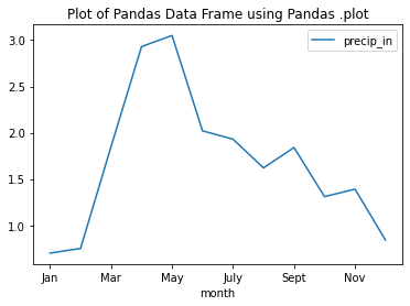
A Quick Plot
You can plot pandas dataframe using matplotlib or using the pandas .plot() method which wraps around matplotlib.
f, ax = plt.subplots()
avg_monthly_precip.plot(x="month",
                        y="precip_in",
                        title="Plot of Pandas Data Frame using Pandas .plot",
                        ax=ax)
plt.show()
/opt/conda/lib/python3.8/site-packages/pandas/plotting/_matplotlib/core.py:1235: UserWarning: FixedFormatter should only be used together with FixedLocator
  ax.set_xticklabels(xticklabels)
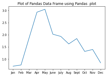
Or you can plot using the standard matplotlib approach. In this course we will encourage you to use the matplotlib approach which will be more flexible as you begin to create more complex plots.
f, ax = plt.subplots()
ax.plot(avg_monthly_precip.month,
        avg_monthly_precip.precip_in)

ax.set(title="Plot of Pandas Data Frame using Pandas .plot")
plt.show()
In the pages that follow, you will learn how to import data from .csv files into pandas dataframes, run calculations and summary statistics on pandas dataframes, and select data from pandas dataframes.
Share on
Twitter Facebook Google+ LinkedIn
Leave a Comment