Lesson 2. GIS in Python: Intro to Coordinate Reference Systems in Python
Learning Objectives
- Be able to describe what a Coordinate Reference System (
CRS) is. - Be able to list the steps associated with plotting 2 datasets stored using different coordinate reference systems.
Intro to Coordinate Reference Systems
The short video below highlights how map projections can make continents look proportionally larger or smaller than they actually are.
What is a Coordinate Reference System
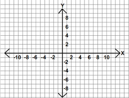
To define the location of something you often use a coordinate system. This system consists of an X and a Y value located within a 2 (or more) -dimensional space.
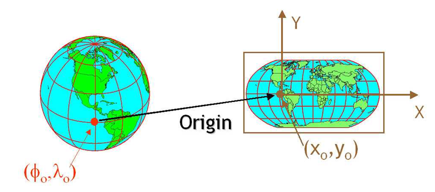
While the above coordinate system is 2-dimensional, you live on a 3-dimensional earth that happens to be “round”. To define the location of objects on the earth, which is round, you need a coordinate system that adapts to the Earth’s shape. When you make maps on paper or on a flat computer screen, you move from a 3-Dimensional space (the globe) to a 2-Dimensional space (your computer screens or a piece of paper). The components of the CRS define how the “flattening” of data that exists in a 3-D globe space. The CRS also defines the the coordinate system itself.
A coordinate reference system (CRS) is a coordinate-based local, regional or global system used to locate geographical entities. – Wikipedia
The Components of a CRS
The coordinate reference system is made up of several key components:
- Coordinate System: the X, Y grid upon which your data is overlayed and how you define where a point is located in space.
- Horizontal and vertical units: The units used to define the grid along the x, y (and z) axis.
- Datum: A modeled version of the shape of the earth which defines the origin used to place the coordinate system in space. You will explain this further, below.
- Projection Information: the mathematical equation used to flatten objects that are on a round surface (e.g. the earth) so you can view them on a flat surface (e.g. your computer screens or a paper map).
Why CRS is Important
It is important to understand the coordinate system that your data uses - particularly if you are working with different data stored in different coordinate systems. If you have data from the same location that are stored in different coordinate reference systems, they will not line up in any GIS or other program unless you have a program like ArcGIS or QGIS that supports projection on the fly. Even if you work in a tool that supports projection on the fly, you will want all of your data in the same projection for performing analysis and processing tasks.
Data Tip: Spatialreference.org provides an excellent online library of CRS information.
Coordinate System & Units
You can define a spatial location, such as a plot location, using an x- and a y-value - similar to your cartesian coordinate system displayed in the figure, above.
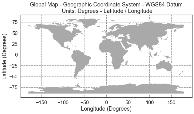
For example, the map below shows all of the continents in the world, in a Geographic Coordinate Reference System. The units are Degrees and the coordinate system itself is latitude and longitude with the origin being the location where the equator meets the central meridian on the globe (0,0).
Next, you will learn more about CRS by exploring some data. Note that you don’t need to actually submit anything reviewed in this lesson for your homework. It’s just a way to show you how the CRS impacts your data.
import os
import numpy as np
import pandas as pd
import matplotlib.pyplot as plt
from matplotlib.ticker import ScalarFormatter
import seaborn as sns
import geopandas as gpd
from shapely.geometry import Point
import earthpy as et

# Adjust plot font sizes
sns.set(font_scale=1.5)
sns.set_style("white")

# Set working dir & get data
data = et.data.get_data('spatial-vector-lidar')
os.chdir(os.path.join(et.io.HOME, 'earth-analytics'))
To begin, load a shapefile using geopandas.
# Import world boundary shapefile
worldBound_path = os.path.join("data", "spatial-vector-lidar", "global",
                               "ne_110m_land", "ne_110m_land.shp")
worldBound = gpd.read_file(worldBound_path)
Plot the Data
# Plot worldBound data using geopandas
fig, ax = plt.subplots(figsize=(10, 5))
worldBound.plot(color='darkgrey',
                ax=ax)
# Set the x and y axis labels
ax.set(xlabel="Longitude (Degrees)",
       ylabel="Latitude (Degrees)",
       title="Global Map - Geographic Coordinate System - WGS84 Datum\n Units: Degrees - Latitude / Longitude")

# Add the x y graticules
ax.set_axisbelow(True)
ax.yaxis.grid(color='gray',
              linestyle='dashed')
ax.xaxis.grid(color='gray',
              linestyle='dashed')
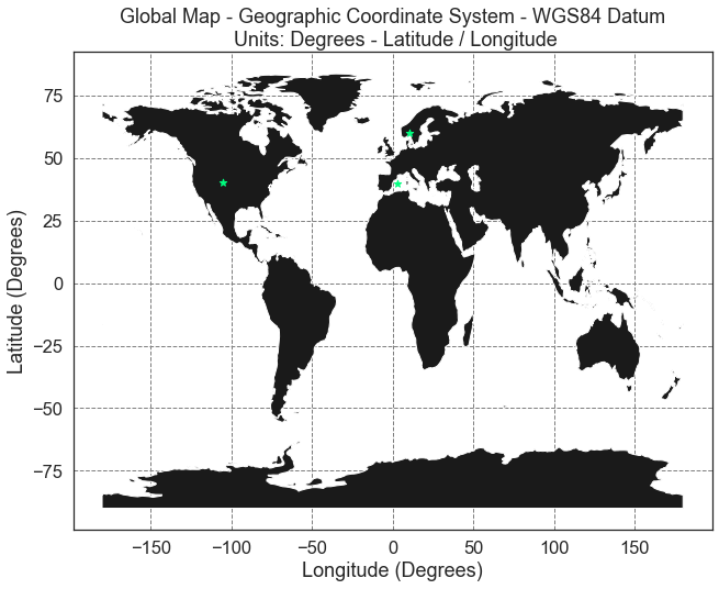
Create Spatial Points Object
Next, add three coordinate locations to your map. Note that the UNITS are in decimal degrees (latitude, longitude):
- Boulder, Colorado: 40.0274, -105.2519
- Oslo, Norway: 59.9500, 10.7500
- Mallorca, Spain: 39.6167, 2.9833
To plot these points spatially you will
- create a numpy array of the point locations and
- Use a for loop to populate a
shapelyPointobject
# Create numpy array of x,y point locations
add_points = np.array([[-105.2519,   40.0274],
                       [  10.75  ,   59.95  ],
                       [   2.9833,   39.6167]])

# Turn points into list of x,y shapely points
city_locations = [Point(xy) for xy in add_points]
city_locations
[<shapely.geometry.point.Point at 0x7fb0b90558b0>,
 <shapely.geometry.point.Point at 0x7fb0b9055910>,
 <shapely.geometry.point.Point at 0x7fb0b9055970>]
# Create geodataframe using the points
city_locations = gpd.GeoDataFrame(city_locations,
                                  columns=['geometry'],
                                  crs=worldBound.crs)
city_locations.head(3)
| geometry | |
|---|---|
| 0 | POINT (-105.25190 40.02740) |
| 1 | POINT (10.75000 59.95000) |
| 2 | POINT (2.98330 39.61670) |
Finally you can plot the points on top of your world map. Does it look right?
# Plot point locations
fig, ax = plt.subplots(figsize=(12, 8))

worldBound.plot(figsize=(10, 5), color='k',
               ax=ax)
# Add city locations
city_locations.plot(ax=ax,
                    color='springgreen',
                    marker='*',
                    markersize=45)

# Setup x y axes with labels and add graticules
ax.set(xlabel="Longitude (Degrees)", ylabel="Latitude (Degrees)",
       title="Global Map - Geographic Coordinate System - WGS84 Datum\n Units: Degrees - Latitude / Longitude")
ax.set_axisbelow(True)
ax.yaxis.grid(color='gray', linestyle='dashed')
ax.xaxis.grid(color='gray', linestyle='dashed')
Next, import proper graticules that can be projected into a particular coordinate reference system.
# Import graticule & world bounding box shapefile data
graticule_path = os.path.join("data", "spatial-vector-lidar", "global",
                              "ne_110m_graticules_all", "ne_110m_graticules_15.shp")
graticule = gpd.read_file(graticule_path)

bbox_path = os.path.join("data", "spatial-vector-lidar", "global",
                         "ne_110m_graticules_all", "ne_110m_wgs84_bounding_box.shp")
bbox = gpd.read_file(bbox_path)

# Create map axis object
fig, ax = plt.subplots(1, 1, figsize=(15, 8))

# Add bounding box and graticule layers
bbox.plot(ax=ax, alpha=.1, color='grey')
graticule.plot(ax=ax, color='lightgrey')
worldBound.plot(ax=ax, color='black')

# Add points to plot
city_locations.plot(ax=ax,
                    markersize=60,
                    color='springgreen',
                    marker='*')
# Add title and axes labels
ax.set(title="World Map - Geographic Coordinate Reference System (long/lat degrees)",
       xlabel="X Coordinates (meters)",
       ylabel="Y Coordinates (meters)");
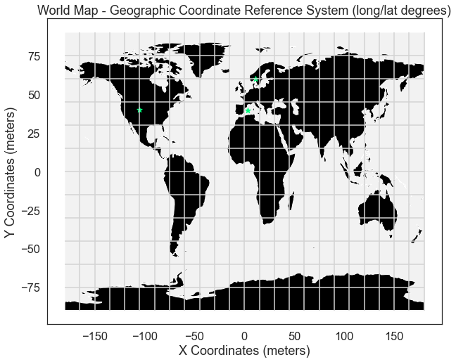
Geographic CRS - The Good & The Less Good
Geographic coordinate systems in decimal degrees are helpful when you need to locate places on the Earth. However, latitude and longitude locations are not located using uniform measurement units. Thus, geographic CRSs are not ideal for measuring distance. This is why other projected CRS have been developed.
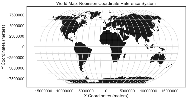
Projected CRS - Robinson
You can view the same data above, in another CRS - Robinson. Robinson is a projected CRS. Notice that the country boundaries on the map - have a different shape compared to the map that you created above in the CRS: Geographic lat/long WGS84.
Below you first reproject your data into the robinson projects (+proj=robin). Then you plot the data once again.
# Reproject the data
worldBound_robin = worldBound.to_crs('+proj=robin')
graticule_robin = graticule.to_crs('+proj=robin')

# Plot the data
fig, ax = plt.subplots(figsize=(12, 8))

worldBound_robin.plot(ax=ax,
                      color='k')

graticule_robin.plot(ax=ax, color='lightgrey')

ax.set(title="World Map: Robinson Coordinate Reference System",
       xlabel="X Coordinates (meters)",
       ylabel="Y Coordinates (meters)")

for axis in [ax.xaxis, ax.yaxis]:
    formatter = ScalarFormatter()
    formatter.set_scientific(False)
    axis.set_major_formatter(formatter)
What happens if you add the same Lat / Long coordinate locations that you used above, to your map? Remember that the data on your map are in the CRS - Robinson.
# Plot the data
fig, ax = plt.subplots(1, 1, figsize=(12, 8))

worldBound_robin.plot(ax=ax,
                      color='k')
graticule_robin.plot(ax=ax,
                     color='lightgrey')
city_locations.plot(ax=ax,
                    marker='*',
                    color='springgreen',
                    markersize=100)

ax.set(title="World Map: Robinson Coordinate Reference System",
       xlabel="X Coordinates (meters)",
       ylabel="Y Coordinates (meters)")

for axis in [ax.xaxis, ax.yaxis]:
    formatter = ScalarFormatter()
    formatter.set_scientific(False)
    axis.set_major_formatter(formatter)

plt.axis('equal');
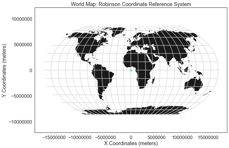
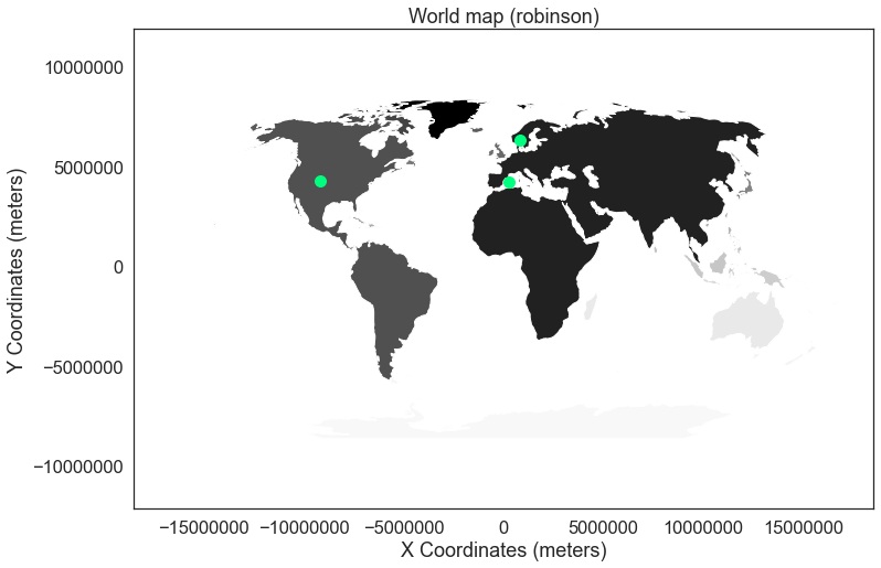
Notice above that when you try to add lat/long coordinates in degrees, to a map in a different CRS, the points are not in the correct location. You need to first convert the points to the same CRS that your other data are in. The process of converting a dataset from one CRS to another is often referred to as reprojection.
In python, you use the .to_crs method to reproject your data.
# Reproject point locations to the Robinson projection
city_locations_robin = city_locations.to_crs(worldBound_robin.crs)

fig, ax = plt.subplots(1, 1, figsize=(12, 8))
worldBound_robin.plot(ax=ax,
                      cmap='Greys')
ax.set(title="World map (robinson)",
       xlabel="X Coordinates (meters)",
       ylabel="Y Coordinates (meters)")
city_locations_robin.plot(ax=ax, markersize=100, color='springgreen')

for axis in [ax.xaxis, ax.yaxis]:
    formatter = ScalarFormatter()
    formatter.set_scientific(False)
    axis.set_major_formatter(formatter)

plt.axis('equal');
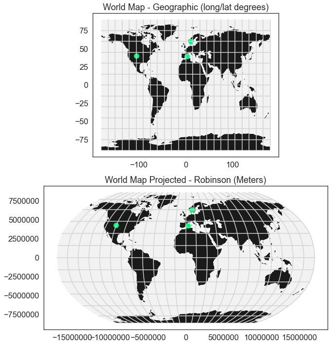
Compare Maps
Both of the plots above look visually different and also use a different coordinate system. Look at both, side by side, with the actual graticules or latitude and longitude lines rendered on the map.
# Reproject graticules and bounding box  to robinson
graticule_robinson = graticule.to_crs('+proj=robin')
bbox_robinson = bbox.to_crs('+proj=robin')

# Setup plot with 2 "rows" one for each map and one column
fig, (ax0, ax1) = plt.subplots(2, 1, figsize=(13, 12))

# First plot
bbox.plot(ax=ax0,
          alpha=.1,
          color='grey')

graticule.plot(ax=ax0,
               color='lightgrey')

worldBound.plot(ax=ax0,
                color='k')

city_locations.plot(ax=ax0,
                    markersize=100,
                    color='springgreen')

ax0.set(title="World Map - Geographic (long/lat degrees)")

# Second plot
bbox_robinson.plot(ax=ax1,
                   alpha=.1,
                   color='grey')

graticule_robinson.plot(ax=ax1,
                        color='lightgrey')

worldBound_robin.plot(ax=ax1,
                      color='k')

city_locations_robin.plot(ax=ax1,
                          markersize=100,
                          color='springgreen')

ax1.set(title="World Map Projected - Robinson (Meters)")

for axis in [ax1.xaxis, ax1.yaxis]:
    formatter = ScalarFormatter()
    formatter.set_scientific(False)
    axis.set_major_formatter(formatter)
Why Multiple CRS?
You may be wondering, why bother with different CRSs if it makes your analysis more complicated? Well, each CRS is optimized to best represent the:
- shape and/or
- scale / distance and/or
- area
of features in the data. And no one CRS is great at optimizing all three elements: shape, distance AND area. Some CRSs are optimized for shape, some are optimized for distance and some are optimized for area. Some CRSs are also optimized for particular regions - for instance the United States, or Europe. Discussing CRS as it optimizes shape, distance and area is beyond the scope of this tutorial, but it’s important to understand that the CRS that you chose for your data, will impact working with the data.
We will discuss some of the differences between the projected UTM CRS and geographic WGS84 in the next lesson.
Challenge
Compare the maps of the globe above. What do you notice about the shape of the various countries. Are there any signs of distortion in certain areas on either map? Which one is better?
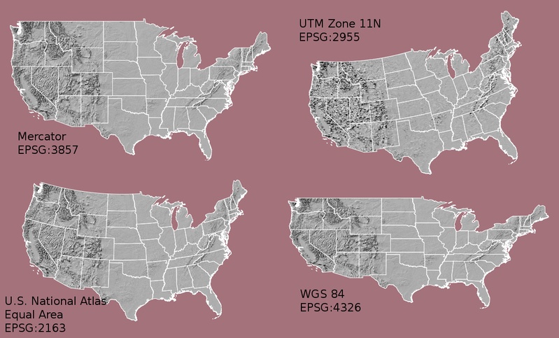
Look at the image below which depicts maps of the United States in 4 different
CRSs. What visual differences do you notice in each map? Look up each projection online, what elements (shape,area or distance) does each projection used in the graphic below optimize?
Geographic vs. Projected CRS
The above maps provide examples of the two main types of coordinate systems:
- Geographic coordinate systems: coordinate systems that span the entire globe (e.g. latitude / longitude).
- Projected coordinate Systems: coordinate systems that are localized to minimize visual distortion in a particular region (e.g. Robinson, UTM, State Plane)
You will discuss these two coordinate reference systems types in more detail in the next lesson.
Additional Resources
- Read more on coordinate systems in the QGIS documentation.
- For more on the types of projections, visit ESRI’s ArcGIS reference on projection types..
- Read more about choosing a projection/datum.
Share on
Twitter Facebook Google+ LinkedIn
Leave a Comment