In the last lesson, you reviewed the basic principles behind what a lidar raster dataset is in R and how point clouds are used to derive the raster. In this lesson, you will learn how to open and plot a lidar raster dataset in R. You will also learn 3 key attributes of a raster dataset:

1. Spatial resolution
2. Spatial extent
3. Coordinate reference system

Open Raster Data in R

To work with raster data in R, you can use the raster and rgdal packages.

# load libraries
library(raster)
library(rgdal)

# Make sure your working directory is set to  wherever your 'earth-analytics' dir is
# setwd("earth-analytics-dir-path-here")

You use the raster("path-to-raster-here") function to open a raster dataset in R. Note that you use the plot() function to plot the data. The function argument main = "" adds a title to the plot.

# open raster data
lidar_dem <- raster(x = "data/week-03/BLDR_LeeHill/pre-flood/lidar/pre_DTM.tif")

# plot raster data
plot(lidar_dem,
     main = "Digital Elevation Model - Pre 2013 Flood")

If you zoom in on a small section of the raster, you can see the individual pixels that make up the raster. Each pixel has one value associated with it. In this case that value represents the elevation of ground.

Note that you are using the xlim= argument to zoom in to on region of the raster. You can use xlim and ylim to define the x and y axis extents for any plot.

# zoom in to one region of the raster
plot(lidar_dem,
  xlim = c(473000, 473030), # define the x limits
  ylim = c(4434000, 4434030), # define y limits for the plot
     main = "Lidar Raster - Zoomed into one small region")

Next, let’s discuss some of the important spatial attributes associated with raster data.

1. Coordinate Reference System

The coordinate reference system (CRS) of a spatial object tells R where the raster is located in geographic space. It also tells R what method should be used to “flatten” or project the raster in geographic space.

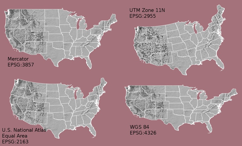
What Makes Spatial Data Line Up on a Map?

You will learn CRS in more detail in next weeks class. For this week, just remember that data from the same location but saved in different coordinate references systems will not line up in any GIS or other program. Thus, it’s important when working with spatial data in a program like R to identify the coordinate reference system applied to the data and retain it throughout data processing and analysis.

View Raster CRS in R

You can view the CRS string associated with your R object using thecrs() method. You can assign this string to an R object too.

# view resolution units
crs(lidar_dem)
## CRS arguments:
##  +proj=utm +zone=13 +datum=WGS84 +units=m +no_defs +ellps=WGS84
## +towgs84=0,0,0

# assign crs to an object (class) to use for reprojection and other tasks
myCRS <- crs(lidar_dem)
myCRS
## CRS arguments:
##  +proj=utm +zone=13 +datum=WGS84 +units=m +no_defs +ellps=WGS84
## +towgs84=0,0,0

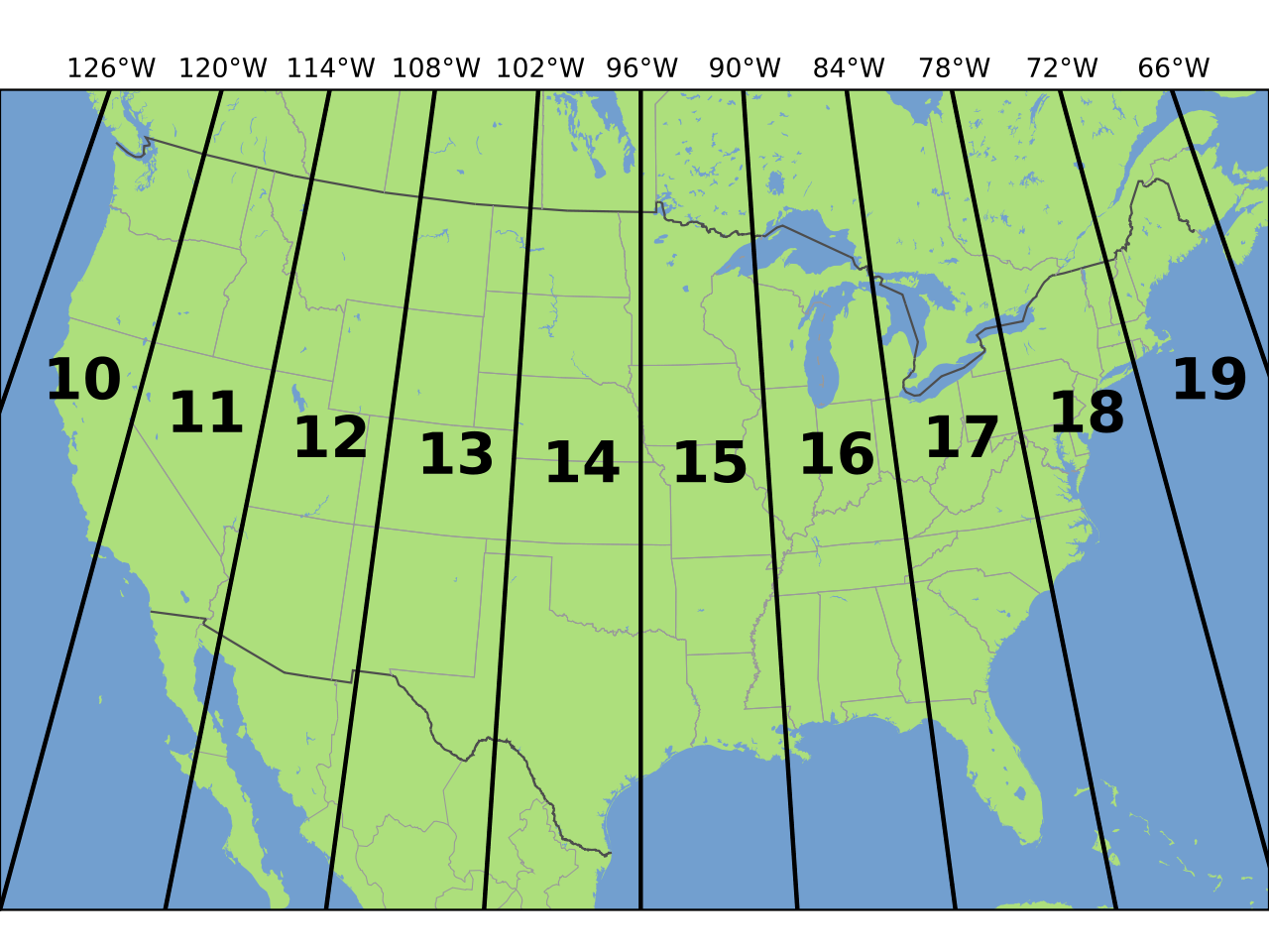
The CRS string for our lidar_dem object tells us that your data are in the UTM projection.

The CRS format, returned by R, is in a PROJ 4 format. This means that the projection information is strung together as a series of text elements, each of which begins with a + sign.

+proj=utm +zone=18 +datum=WGS84 +units=m +no_defs +ellps=WGS84 +towgs84=0,0,0

You’ll focus on the first few components of the CRS in this tutorial.

• +proj=utm The projection of the dataset. Your data are in Universal Transverse Mercator (UTM).
• +zone=18 The UTM projection divides up the world into zones, this element tells you which zone the data is in. Harvard Forest is in Zone 18.
• +datum=WGS84 The datum was used to define the center point of the projection. Your raster uses the WGS84 datum.
• +units=m This is the horizontal units that the data are in. Your units are meters.

Spatial Extent

Next, let’s discuss spatial extent. The spatial extent of a raster or spatial object is the geographic area that the raster data covers.

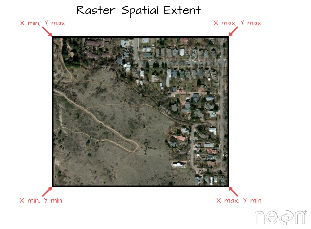
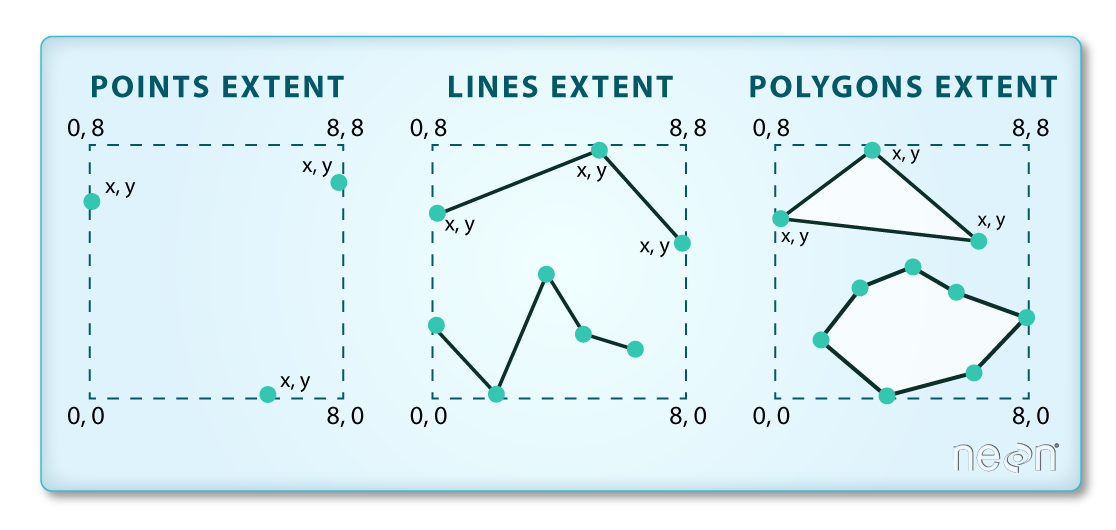
The spatial extent of an R spatial object represents the geographic “edge” or location that is the furthest north, south, east and west. In other words, extent represents the overall geographic coverage of the spatial object.

Raster Resolution

A raster has horizontal (x and y) resolution. This resolution represents the area on the ground that each pixel covers. The units for your data are in meters. In this case, your data resolution is 1 x 1. This means that each pixel represents a 1 x 1 meter area on the ground. You can figure out the units of this resolution using the crs() function which you will use next.

# what is the x and y resolution for your raster data?
xres(lidar_dem)
## [1] 1
yres(lidar_dem)
## [1] 1

Resolution Units

Resolution as a number doesn’t mean anything unless you know the units. You can figure out the horizontal (x and y) units from the coordinate reference system string.

# view coordinate reference system
crs(lidar_dem)
## CRS arguments:
##  +proj=utm +zone=13 +datum=WGS84 +units=m +no_defs +ellps=WGS84
## +towgs84=0,0,0

Notice this string contains an element called units=m. This means the units are in meters. You won’t get into too much detail about coordinate reference strings in this weeks class but they are important to be familiar with when working with spatial data. You will learn them in more detail during the semester!