Mapping migration

Introduction to vector data operations

Learning Goals:

Combine different types of vector data with spatial joins
Create a chloropleth plot

The Veery thrush (Catharus fuscescens) migrates each year between nesting sites in the U.S. and Canada, and South America. Veeries are small birds, and encountering a hurricane during their migration would be disasterous. However, Ornithologist Christopher Hechscher has found in tracking their migration that their breeding patterns and migration timing can predicting the severity of hurricane season as accurately as meterological models (Heckscher, 2018)!

Veery in Central Park by the Ramble Stone Arch. Source: Wikimedia

You can read more about the Veery migration and how climate change may be impacting these birds in this article from the Audobon Society, or in Heckscher’s open access report.

Check out our demo video!

DEMO: Migration Part 1 (EDA) by Earth Lab

DEMO: Migration Part 2 (EDA) by Earth Lab

DEMO: Migration Part 3 (EDA) by Earth Lab

Reflect and Respond: What can we learn from migration patterns?

Reflect on what you know about migration. You could consider:

What are some reasons that animals migrate?
How might climate change affect animal migrations?
Do you notice any animal migrations in your area?

id = 'eda'
project_title = 'Veery Migration 2023'
species_name = 'Veery thrush'
species_lookup = 'catharus fuscescens'
year = 2023
gbif_filename = 'gbif_veery.csv'
ecoregions_dir = 'ecoregions'
plot_filename = 'veery_migration'
plot_height = 800

STEP 1: Set up your reproducible workflow

Import Python libraries

Try It: Import packages

In the imports cell, we’ve included some packages that you will need. Add imports for packages that will help you:

Work with tabular data
Work with geospatial vector data

import os
import pathlib

import earthpy

Create a directory for your data

For this challenge, you will need to download some data to the computer you’re working on. We suggest using the earthpy library we develop to manage your downloads, since it encapsulates many best practices as far as:

Where to store your data
Dealing with archived data like .zip files
Avoiding version control problems
Making sure your code works cross-platform
Avoiding duplicate downloads

If you’re working on one of our assignments through GitHub Classroom, it also lets us build in some handy defaults so that you can see your data files while you work.

Try It: Create a project folder

The code below will help you get started with making a project directory

Replace 'your-project-directory-name-here' with a descriptive name
Run the cell
The code should have printed out the path to your data files. Check that your data directory exists and has data in it using the terminal or your Finder/File Explorer.

File structure

These days, a lot of people find your file by searching for them or selecting from a Bookmarks or Recents list. Even if you don’t use it, your computer also keeps files in a tree structure of folders. Put another way, you can organize and find files by travelling along a unique path, e.g. My Drive > Documents > My awesome project > A project file where each subsequent folder is inside the previous one. This is convenient because all the files for a project can be in the same place, and both people and computers can rapidly locate files they want, provided they remember the path.

You may notice that when Python prints out a file path like this, the folder names are separated by a / or \ (depending on your operating system). This character is called the file separator, and it tells you that the next piece of the path is inside the previous one.

# Create data directory
project = earthpy.Project(
    title=project_title,
    dirname='your-project-directory-name-here')
# Download sample data
project.get_data()

# Display the project directory
project.project_dir

Downloading from https://ndownloader.figshare.com/files/58363291
Downloading from https://ndownloader.figshare.com/files/58369498
Extracted output to /home/runner/.local/share/earth-analytics/veery-migration-2023/ecoregions

PosixPath('/home/runner/.local/share/earth-analytics/veery-migration-2023')

STEP 2: Define your study area – the ecoregions of North America

Your sample data package included a Shapefile of global ecoregions. You should be able to see changes in the number of observations of Veery thrush in each ecoregion throughout the year.

You don’t have to use ecoregions to group species observations – you could choose to use political boundaries like countries or states, other natural boundaries like watersheds, or even uniform hexagonal areas as is common in conservation work. We chose ecoregions because we expect the suitability for a species at a particular time of year to be relatively consistent across the region.

The ecoregion data will be available as a shapefile. Learn more about shapefiles and vector data in this Introduction to Spatial Vector Data File Formats in Open Source Python

Load the ecoregions into Python

Try It: Load ecoregions into Python

Download and save ecoregion boundaries from the EPA:

Replace a_path with the path your created for your ecoregions file.
Make a quick plot with .plot() to make sure the download worked.

# Open up the ecoregions boundaries
gdf = gpd.read_file(a_path)

# Plot the ecoregions quickly to check download

ERROR 1: PROJ: proj_create_from_database: Open of /usr/share/miniconda/envs/learning-portal/share/proj failed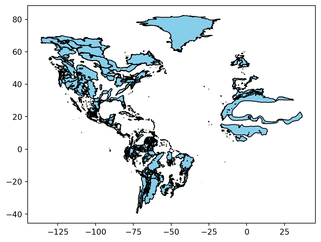

STEP 3: Load species observation data

For this challenge, you will use a database called the Global Biodiversity Information Facility (GBIF). GBIF is compiled from species observation data all over the world, and includes everything from museum specimens to photos taken by citizen scientists in their backyards. We’ve compiled some sample data in the same format that you will get from GBIF.

Let’s start by looking at a little of the raw data.

gbif_path = project.project_dir / gbif_filename

Try It: Load GBIF data

Look at the beginning of the file you downloaded using the code below. What do you think the delimiter is?
Run the following code cell. What happens?
Uncomment and modify the parameters of pd.read_csv() below until your data loads successfully and you have only the columns you want.

You can use the following code to look at the beginning of your file:

!head -n 2 $gbif_path

gbifID  datasetKey  occurrenceID    kingdom phylum  class   order   family  genus   species infraspecificEpithet    taxonRank   scientificName  verbatimScientificName  verbatimScientificNameAuthorship    countryCode locality    stateProvince   occurrenceStatus    individualCount publishingOrgKey    decimalLatitude decimalLongitude    coordinateUncertaintyInMeters   coordinatePrecision elevation   elevationAccuracy   depth   depthAccuracy   eventDate   day month   year    taxonKey    speciesKey  basisOfRecord   institutionCode collectionCode  catalogNumber   recordNumber    identifiedBy    dateIdentified  license rightsHolder    recordedBy  typeStatus  establishmentMeans  lastInterpreted mediaType   issue
4158712344  8a863029-f435-446a-821e-275f4f641165    https://observation.org/observation/273993634   Animalia    Chordata    Aves    Passeriformes   Turdidae    Catharus    Catharus fuscescens     SPECIES Catharus fuscescens (Stephens, 1817)    Catharus fuscescens     CA  Ontario - Point Pelee NP    Ontario PRESENT 1   c8d737e0-2ff8-42e8-b8fc-6b805d26fc5f    41.9137 -82.5092    8.0                     2023-05-19  19  5   2023    2490804 2490804 HUMAN_OBSERVATION                           CC_BY_NC_4_0    Stichting Observation International User 1751           2025-09-24T01:21:44.728Z

# Load the GBIF data
gbif_df = pd.read_csv(
    gbif_path, 
    delimiter='',
    index_col='',
    usecols=[]
)
gbif_df.head()

	decimalLatitude	decimalLongitude	month
gbifID
4158712344	41.913700	-82.509200	5
4923515059	41.852812	-87.611721	5
4923522410	41.852812	-87.611721	9
4923520798	41.852812	-87.611721	5
4923520314	41.880356	-87.630134	9

Convert the GBIF data to a GeoDataFrame

To plot the GBIF data, we need to convert it to a GeoDataFrame first. This will make some special geospatial operations from geopandas available, such as spatial joins and plotting.

Try It: Convert `DataFrame` to `GeoDataFrame`

Replace your_dataframe with the name of the DataFrame you just got from GBIF
Replace longitude_column_name and latitude_column_name with column names from your `DataFrame
Run the code to get a GeoDataFrame of the GBIF data.

gbif_gdf = (
    gpd.GeoDataFrame(
        your_dataframe, 
        geometry=gpd.points_from_xy(
            your_dataframe.longitude_column_name, 
            your_dataframe.latitude_column_name), 
        crs="EPSG:4326")
    # Select the desired columns
    [[]]
)
gbif_gdf

	month	geometry
gbifID
4158712344	5	POINT (-82.5092 41.9137)
4923515059	5	POINT (-87.61172 41.85281)
4923522410	9	POINT (-87.61172 41.85281)
4923520798	5	POINT (-87.61172 41.85281)
4923520314	9	POINT (-87.63013 41.88036)
...	...	...
4423534780	9	POINT (-75.1254 40.0626)
4524632357	6	POINT (-89.8049 44.6967)
4173211734	5	POINT (-82.4753 42.0478)
4173216429	6	POINT (-74.5468 46.1638)
4423531794	9	POINT (-75.1254 40.0626)

165614 rows × 2 columns

STEP 4: Count the number of observations in each ecosystem, during each month of 2023

Much of the data in GBIF is crowd-sourced. As a result, we need not just the number of observations in each ecosystem each month – we need to normalize by some measure of sampling effort. After all, we wouldn’t expect the same number of observations at the North Pole as we would in a National Park, even if there were the same number organisms. In this case, we’re normalizing using the average number of observations for each ecosystem and each month. This should help control for the number of active observers in each location and time of year.

Identify the ecoregion for each observation

You can combine the ecoregions and the observations spatially using a method called .sjoin(), which stands for spatial join.

Check out the geopandas documentation on spatial joins to help you figure this one out. You can also ask your favorite LLM (Large-Language Model, like ChatGPT)

Try It: Perform a spatial join

Identify the correct values for the how= and predicate= parameters of the spatial join.

gbif_ecoregion_gdf = (
    ecoregions_gdf
    # Match the CRS of the GBIF data and the ecoregions
    .to_crs(gbif_gdf.crs)
    # Find ecoregion for each observation
    .sjoin(
        gbif_gdf,
        how='', 
        predicate='')
)
gbif_ecoregion_gdf

	eco_code	area_km2	geometry	gbifID	month
12	NA0517	133597	POLYGON ((-76.11368 38.88879, -76.11789 38.885...	4734332451	5
13	NA0411	89778	POLYGON ((-71.99018 41.28049, -71.98594 41.279...	4739064468	5
13	NA0411	89778	POLYGON ((-71.99018 41.28049, -71.98594 41.279...	4767578666	5
13	NA0411	89778	POLYGON ((-71.99018 41.28049, -71.98594 41.279...	4821324417	5
13	NA0411	89778	POLYGON ((-71.99018 41.28049, -71.98594 41.279...	4816544303	5
...	...	...	...	...	...
1977	NA0602	463345	POLYGON ((-91.84863 54.90782, -91.86077 54.936...	5689247856	7
1979	NA0504	8975	POLYGON ((-69.99612 41.56885, -69.99683 41.577...	4648000283	9
1979	NA0504	8975	POLYGON ((-69.99612 41.56885, -69.99683 41.577...	4612716677	9
1984	NA0517	133597	POLYGON ((-77.91596 34.04894, -77.91089 34.052...	4719091123	9
1984	NA0517	133597	POLYGON ((-77.91596 34.04894, -77.91089 34.052...	4664856615	9

126372 rows × 5 columns

Count the observations in each ecoregion each month

Try It: Group observations by ecoregion

Replace columns_to_group_by with a list of columns. Keep in mind that you will end up with one row for each group – you want to count the observations in each ecoregion by month.
Select only month/ecosystem combinations that have more than one occurrence recorded, since a single occurrence could be an error.
Use the .groupby() and .mean() methods to compute the mean occurrences by ecoregion and by month.
Run the code – it will normalize the number of occurrences by month and ecoretion.

occurrence_df = (
    gbif_ecoregion_gdf
    # Select only necessary columns
    [[]]
    # For each ecoregion, for each month...
    .groupby(columns_to_group_by)
    # ...count the number of occurrences
    .agg(occurrences=('name', 'count'))
)

# Get rid of rare observations (possible misidentification?)
occurrence_df = occurrence_df[...]

# Take the mean by ecoregion
mean_occurrences_by_ecoregion = (
    occurrence_df
    ...
)
# Take the mean by month
mean_occurrences_by_month = (
    occurrence_df
    ...
)

Normalize the observations

Try It: Normalize

Divide occurrences by the mean occurrences by month AND the mean occurrences by ecoregion

# Normalize by space and time for sampling effort
occurrence_df['norm_occurrences'] = (
    occurrence_df
    ...
)
occurrence_df

		gbifID	norm_occurrences
eco_code	month
Lake	4	12	0.000180
	5	1792	0.003530
	6	29	0.000066
	7	29	0.000127
	8	41	0.000426
...	...	...	...
NT0904	5	31	0.000547
	9	63	0.005378
	10	38	0.021693
NT1402	4	6	0.005174
NT1403	10	11	0.021978

170 rows × 2 columns

STEP 5: Plot the Veery thrush observations by month

First thing first – let’s load your stored variables and import libraries.

%store -r ecoregions_gdf occurrence_df

Try It: Import packages

In the imports cell, we’ve included some packages that you will need. Add imports for packages that will help you:

Make interactive maps with vector data

# Get month names
import calendar

# Libraries for Dynamic mapping
import cartopy.crs as ccrs
import panel as pn

Create a simplified `GeoDataFrame` for plotting

Plotting larger files can be time consuming. The code below will streamline plotting with hvplot by simplifying the geometry, projecting it to a Mercator projection that is compatible with geoviews, and cropping off areas in the Arctic.

Try It: Simplify ecoregion data

Download and save ecoregion boundaries from the EPA:

Simplify the ecoregions with .simplify(.05), and save it back to the geometry column.
Change the Coordinate Reference System (CRS) to Mercator with .to_crs(ccrs.Mercator())
Use the plotting code that is already in the cell to check that the plotting runs quickly (less than a minute) and looks the way you want, making sure to change gdf to YOUR GeoDataFrame name.

# Simplify the geometry to speed up processing

# Change the CRS to Mercator for mapping

# Check that the plot runs in a reasonable amount of time
gdf.hvplot(geo=True, crs=ccrs.Mercator())

Try It: Map migration over time

If applicable, replace any variable names with the names you defined previously.
Replace column_name_used_for_ecoregion_color and column_name_used_for_slider with the column names you wish to use.
Customize your plot with your choice of title, tile source, color map, and size.

Note

Your plot will probably still change months very slowly in your Jupyter notebook, because it calculates each month’s plot as needed. Open up the saved HTML file to see faster performance!

# Join the occurrences with the plotting GeoDataFrame
occurrence_gdf = ecoregions_gdf.join(occurrence_df)

# Get the plot bounds so they don't change with the slider
xmin, ymin, xmax, ymax = occurrence_gdf.total_bounds

# Plot occurrence by ecoregion and month
migration_plot = (
    occurrence_gdf
    .hvplot(
        c=column_name_used_for_shape_color,
        groupby=column_name_used_for_slider,
        # Use background tiles
        geo=True, crs=ccrs.Mercator(), tiles='CartoLight',
        title="Your Title Here",
        xlim=(xmin, xmax), ylim=(ymin, ymax),
        frame_height=600,
        widget_location='bottom'
    )
)

# Save the plot
migration_plot.save('migration.html', embed=True)

  0%|          | 0/12 [00:00<?, ?it/s] 25%|██▌       | 3/12 [00:00<00:00,  9.04it/s] 33%|███▎      | 4/12 [00:00<00:01,  5.61it/s] 42%|████▏     | 5/12 [00:00<00:01,  4.89it/s] 50%|█████     | 6/12 [00:01<00:01,  4.39it/s] 58%|█████▊    | 7/12 [00:01<00:01,  3.90it/s] 67%|██████▋   | 8/12 [00:01<00:01,  3.10it/s] 75%|███████▌  | 9/12 [00:02<00:01,  2.86it/s]

WARNING:bokeh.core.validation.check:W-1005 (FIXED_SIZING_MODE): 'fixed' sizing mode requires width and height to be set: figure(id='p6602', ...)

Looking for an Extra Challenge?: Fix the month labels

Notice that the month slider displays numbers instead of the month name. Use pn.widgets.DiscreteSlider() with the options= parameter set to give the months names. You might want to try asking ChatGPT how to do this, or look at the documentation for pn.widgets.DiscreteSlider(). This is pretty tricky!

References

Heckscher, C. M. (2018). A Nearctic-Neotropical Migratory Songbird’s Nesting Phenology and Clutch Size are Predictors of Accumulated Cyclone Energy. Scientific Reports, 8(1), 9899. https://doi.org/10.1038/s41598-018-28302-3

STEP 1: Set up your reproducible workflow

Import Python libraries

Create a directory for your data

STEP 2: Define your study area – the ecoregions of North America

Load the ecoregions into Python

STEP 3: Load species observation data

Convert the GBIF data to a GeoDataFrame

STEP 4: Count the number of observations in each ecosystem, during each month of 2023

Identify the ecoregion for each observation

Count the observations in each ecoregion each month

Normalize the observations

STEP 5: Plot the Veery thrush observations by month

Create a simplified GeoDataFrame for plotting

References

Create a simplified `GeoDataFrame` for plotting