As you learned in the previous lesson, lidar or Light Detection and Ranging is an active remote sensing system that can be used to measure vegetation height across wide areas. If the data are discrete return, lidar point clouds are most commonly derived data product from a lidar system. However, often people work with lidar data in raster format given it’s smaller in size and thus easier to work with. In this lesson, you will import and work with 3 of the most common lidar derived data products in R:

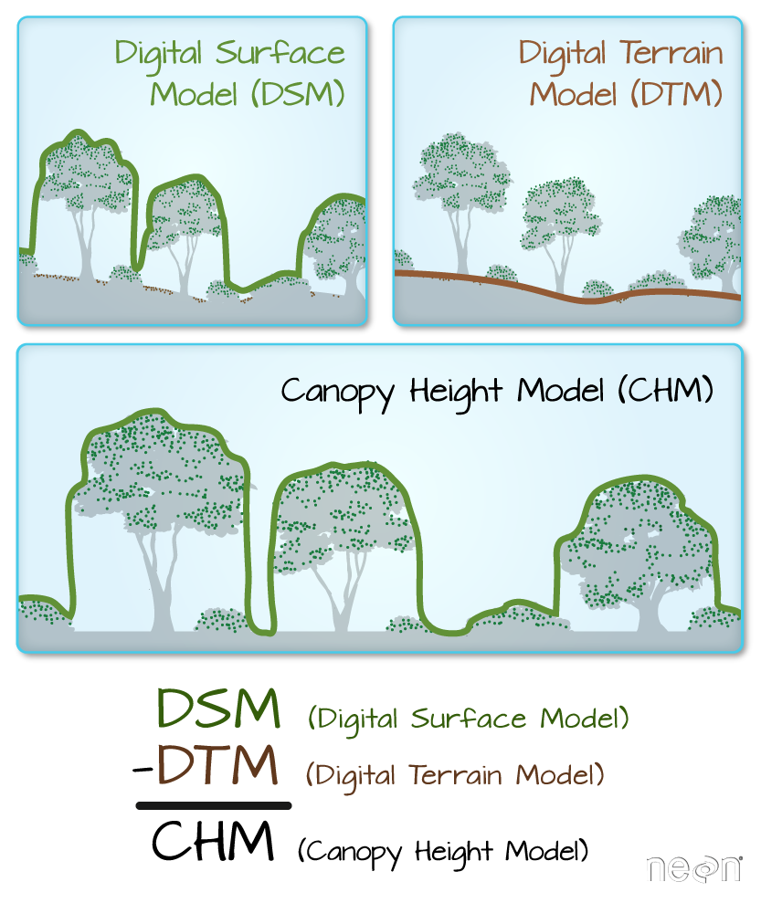
1. Digital Terrain Model (or DTM): ground elevation or the elevation of the Earth’s surface (sometimes also called a DEM or digital elevation model).
2. Digital Surface Model (or DSM): top of the surface (imagine draping a sheet over the canopy of a forest
3. Canopy Height Model (CHM): The height of objects above the ground.

Three Important Lidar Data Products: CHM, DEM, DSM

Digital Elevation Model

In the previous lesson, you opened a digital elevation model. The digital elevation model (DEM), also known as a digital terrain model (DTM) represents the elevation of the Earth’s surface. The DEM represents the ground - and thus DOES NOT INCLUDE trees and buildings and other objects.

# load libraries
library(raster)
library(rgdal)

# set working directory to ensure R can find the file you wish to import
# setwd("working-dir-path-here")

First, let’s open and plot the digital elevation model.

# open raster data
lidar_dem <- raster(x = "data/week-03/BLDR_LeeHill/pre-flood/lidar/pre_DTM.tif")

# plot raster data
plot(lidar_dem,
     main = "Lidar Digital Elevation Model (DEM)")

Next, let’s open the digital SURFACE model (DSM). The DSM represents the top of the earth’s surface. Thus, it INCLUDES TREES, BUILDINGS and other objects that sit on the Earth.

# open raster data
lidar_dsm <- raster(x = "data/week-03/BLDR_LeeHill/pre-flood/lidar/pre_DSM.tif")

# plot raster data
plot(lidar_dsm,
     main = "Lidar Digital Surface Model (DSM)")

Canopy Height Model

The canopy height model (CHM) represents the HEIGHT of the trees. This is not an elevation value, rather it’s the height or distance between the ground and the top of the trees. Some canopy height models also include buildings so you need to look closely at your data to make sure it was properly cleaned before assuming it represents all trees!

Calculate Difference Between Two Rasters

There are different ways to calculate a CHM. One easy way is to subtract the DEM from the DSM.

DSM - DEM = CHM

This math gives you the residual value or difference between the top of the earth surface and the ground which should be the heights of the trees (and buildings if the data haven’t been “cleaned”).

# open raster data
lidar_chm <- lidar_dsm - lidar_dem

# plot raster data
plot(lidar_chm,
     main = "Lidar Canopy Height Model (CHM)")

Plots Using Breaks

Sometimes a gradient of colors is useful to represent a continuous variable. But other times, it’s useful to apply colors to particular ranges of values in a raster. These ranges may be statistically generated or simply visual.

Let’s create breaks in your CHM plot.

# plot raster data
plot(lidar_chm,
     breaks = c(0, 2, 10, 20, 30),
     main = "Lidar Canopy Height Model",
     col = c("white", "brown", "springgreen", "darkgreen"))

Export a Raster

We can export a raster file in R using the write.raster() function. Let’s export the canopy height model that we just created to your data folder. You will create a new directory called “outputs” within the week 3 directory. This structure allows us to keep things organized, separating your outputs from the data you downloaded.

NOTE: You can use the code below to check for and create an outputs directory OR you can create the directory yourself using the finder (MAC) or Windows Explorer.

# check to see if an output directory exists
dir.exists("data/week-03/outputs")
## [1] FALSE

# if the output directory doesn't exist, create it
if (dir.exists("data/week-03/outputs")) {
  print("the directory exists!")
  } else {
    # if the directory doesn't exist, create it
    # recursive tells R to create the entire directory path (data/week-03/outputs)
    dir.create("data/week-03/outputs", recursive = TRUE)
  }

# export CHM object to new GeotIFF
writeRaster(lidar_chm, "data/week-03/outputs/lidar_chm.tiff",
            format = "GTiff",  # output format = GeoTIFF
            overwrite = TRUE) # CAUTION: if this is true, it will overwrite an existing file

# if the output directory doesn't exist, create it
if (!dir.exists("data/week-03/outputs")) {
    # if the directory doesn't exist, create it
    # recursive tells R to create the entire directory path (data/week-03/outputs)
    dir.create("data/week-03/outputs", recursive=TRUE)
}

Change Detection: Terrain

Now that you’ve learned about the three common data products derived from lidar data, let’s use them to do a bit of exploration of your data - as it relates to the 2013 Colorado floods.