Understanding Uncertainty and Error.

It is important to consider error and uncertainty when presenting scientific results. Most measurements that you make - be they from instruments or humans - have uncertainty associated with them. You will learn what that means below.

Uncertainty

Uncertainty: Uncertainty quantifies the range of values within which the value of the measure falls within - within a specified level of confidence. The uncertainty quantitatively indicates the “quality” of your measurement. It answers the question: “how well does the result represent the value of the quantity being measured?”

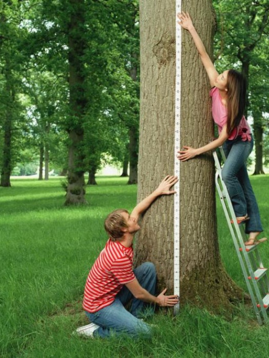
Tree Height Measurement Example

So for example let’s pretend that you measured the height of a tree 10 times. Each time your tree height measurement may be slightly different? Why? Because maybe each time you visually determined the top of the tree to be in a slightly different place. Or maybe there was wind that day during measurements that caused the tree to shift as you measured it yielding a slightly different height each time. or… what other reasons can you think of that might impact tree height measurements?

What is the True Value?

So you may be wondering, what is the true height of your tree? In the case of a tree in a forest, it’s very difficult to determine the true height. So you accept that there will be some variation in your measurements and you measure the tree over and over again until you understand the range of heights that you are likely to get when you measure the tree.

library(raster)
library(rgdal)
# create data frame containing made up tree heights
tree_heights <- data.frame(heights = c(10, 10.1, 9.9, 9.5, 9.7, 9.8,
                                     9.6, 10.5, 10.7, 10.3, 10.6))
# what is the average tree height
mean(tree_heights$heights)
## [1] 10.06364
# what is the standard deviation of measurements?
sd(tree_heights$heights)
## [1] 0.4129715
boxplot(tree_heights$heights,
        main = "Distribution of tree height measurements (m)",
        ylab = "Height (m)",
        col = "springgreen")

In the example above, your mean tree height value is towards the center of your distribution of measured heights. You might expect that the sample mean of your observations provides a reasonable estimate of the true value. The variation among your measured values may also provide some information about the precision (or lack thereof) of the measurement process.

Read more about the basics of a box plot

# view distribution of tree height values
hist(tree_heights$heights, breaks = c(9,9.6,10.4,11),
     main = "Distribution of measured tree height values",
     xlab = "Height (m)", col = "purple")

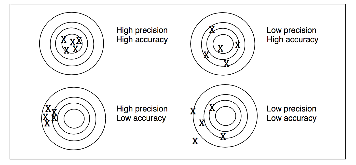
Measurement Accuracy

Measurement accuracy is a concept that relates to whether there is bias in measurements, i.e. whether the expected value of your observations is close to the true value. For low accuracy measurements, you may collect many observations, and the mean of those observations may not provide a good measure of the truth (e.g., the height of the tree). For high accuracy measurements, the mean of many observations would provide a good measure of the true value. This is different from precision, which typically refers to the variation among observations. Accuracy and precision are not always tightly coupled. It is possible to have measurements that are very precise but inaccurate, very imprecise but accurate, etc.

Systematic vs Random Error

Systematic Error: a systematic error is one that tends to shift all measurements in a systematic way. This means that the mean value of a set of measurements is consistently displaced or varied in a predictable way, leading to inaccurate observations. Causes of systematic errors may be known or unknown but should always be corrected for when present. For instance, no instrument can ever be calibrated perfectly, so when a group of measurements systematically differ from the value of a standard reference specimen, an adjustment in the values should be made. Systematic error can be corrected for only when the “true value” (such as the value assigned to a calibration or reference specimen) is known.

Example: Remote sensing instruments need to be calibrated. For example a laser in a lidar system may be tested in a lab to ensure that the distribution of output light energy is consistent every time the laser “fires”.

Random Error: is a component of the total error which, in the course of a number of measurements, varies in an unpredictable way. It is not possible to correct for random error. Random errors can occur for a variety of reasons such as:

• Lack of equipment sensitivity. An instrument may not be able to respond to or indicate a change in some quantity that is too small or the observer may not be able to discern the change.
• Noise in the measurement. Noise is extraneous disturbances that are unpredictable or random and cannot be completely accounted for.
• Imprecise definition. It is difficult to exactly define the dimensions of a object. For example, it is difficult to determine the ends of a crack with measuring its length. Two people may likely pick two different starting and ending points.

Example: Random error may be introduced when you measure tree heights as discussed above.

• Source: nde-ed.org

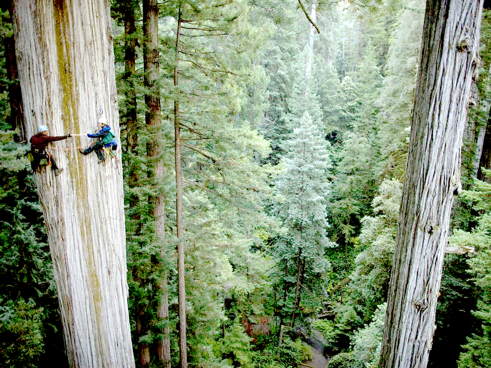
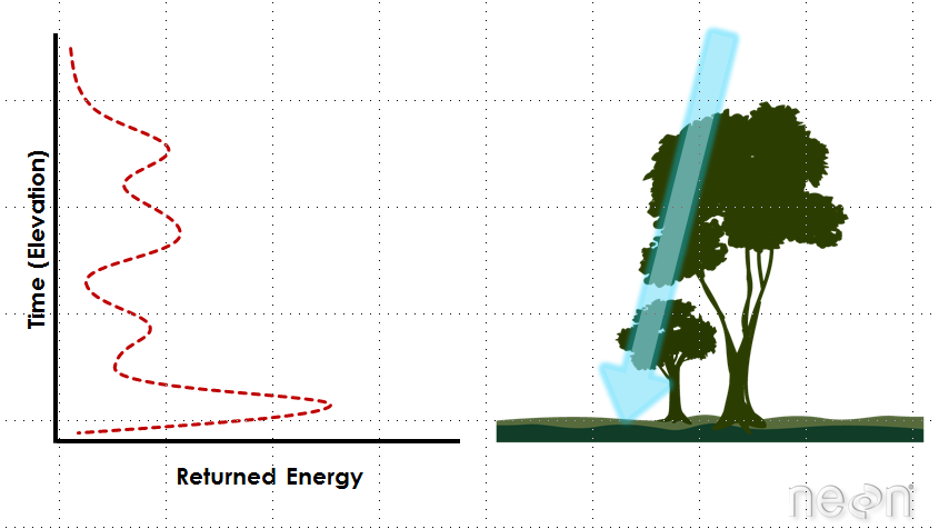
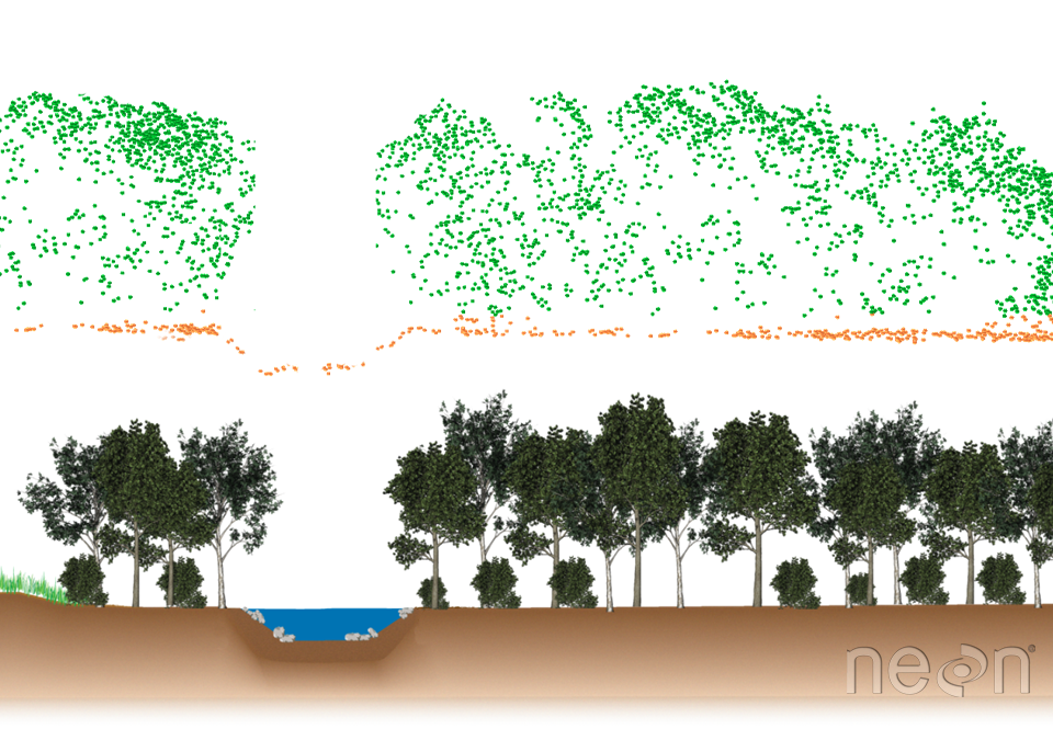
Using Lidar to Estimate Tree Height

You use lidar data to estimate tree height because it is an efficient way to measure large areas of trees (forests) quantitatively. However, you can process the lidar data in many different ways to estimate height. Which method most closely represents the actual heights of the trees on the ground?

Study Site Location

To answer the question above, let’s look at some data from a study site location in California - the San Joaquin Experimental range field site. You can see the field site location on the map below.

Study Area Plots

At this study site, you have both lidar data - specifically a canopy height model that was processed by NEON (National Ecological Observatory Network). You also have some “ground truth” data. That is you have measured tree height values collected at a set of field site plots by technicians at NEON. You call these measured values in situ measurements.

A map of your study plots is below overlaid on top of the canopy height mode.

Compare Lidar Derived Height to In Situ Measurements

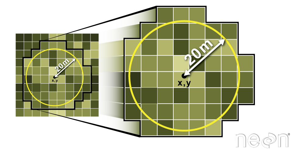
You can compare maximum tree height values at each plot to the maximum pixel value in your CHM for each plot. To do this, you define the geographic boundary of your plot using a polygon - in the case below you use a circle as the boundary. You then extract the raster cell values for each circle and calculate the max value for all of the pixels that fall within the plot area.

Then, you calculate the max height of your measured plot tree height data.

Finally you compare the two using a scatter plot to see how closely the data relate. Do they follow a 1:1 line? Do the data diverge from a 1:1 relationship?

How Different are the Data?

View Interactive Scatterplot

View scatterplot plotly

View Interactive Difference Barplot

View scatterplot differences