Multispectral Imagery in R

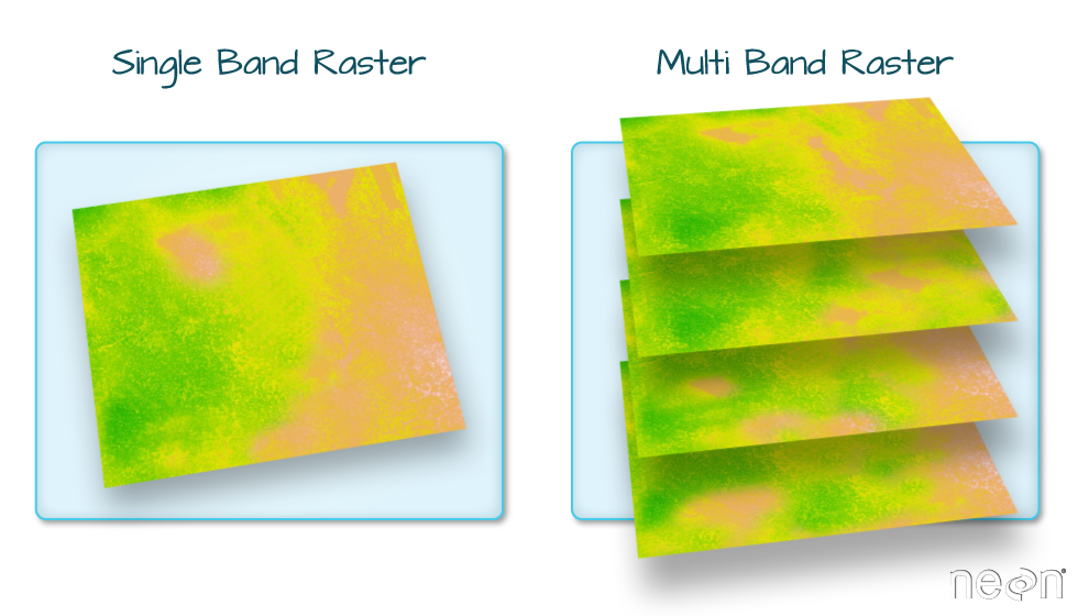
Introduction to Multi-Band Raster Data

In the previous weeks, you have worked with raster data derived from lidar remote sensing instruments. These rasters consisted of one layer or band and contained information height values derived from lidar data. In this lesson, you will learn how to work with rasters containing multispectral imagery data stored within multiple bands (or layers) in R.

Previously, you used the raster() function to open raster data in R. To work with multi-band rasters in R, you need to change how you import and plot your data in several ways.

• To import multi-band raster data you will use the stack() function.
• If your multi-band data are imagery that you wish to composite, you can use plotRGB(), instead of plot(), to plot a 3 band raster image.

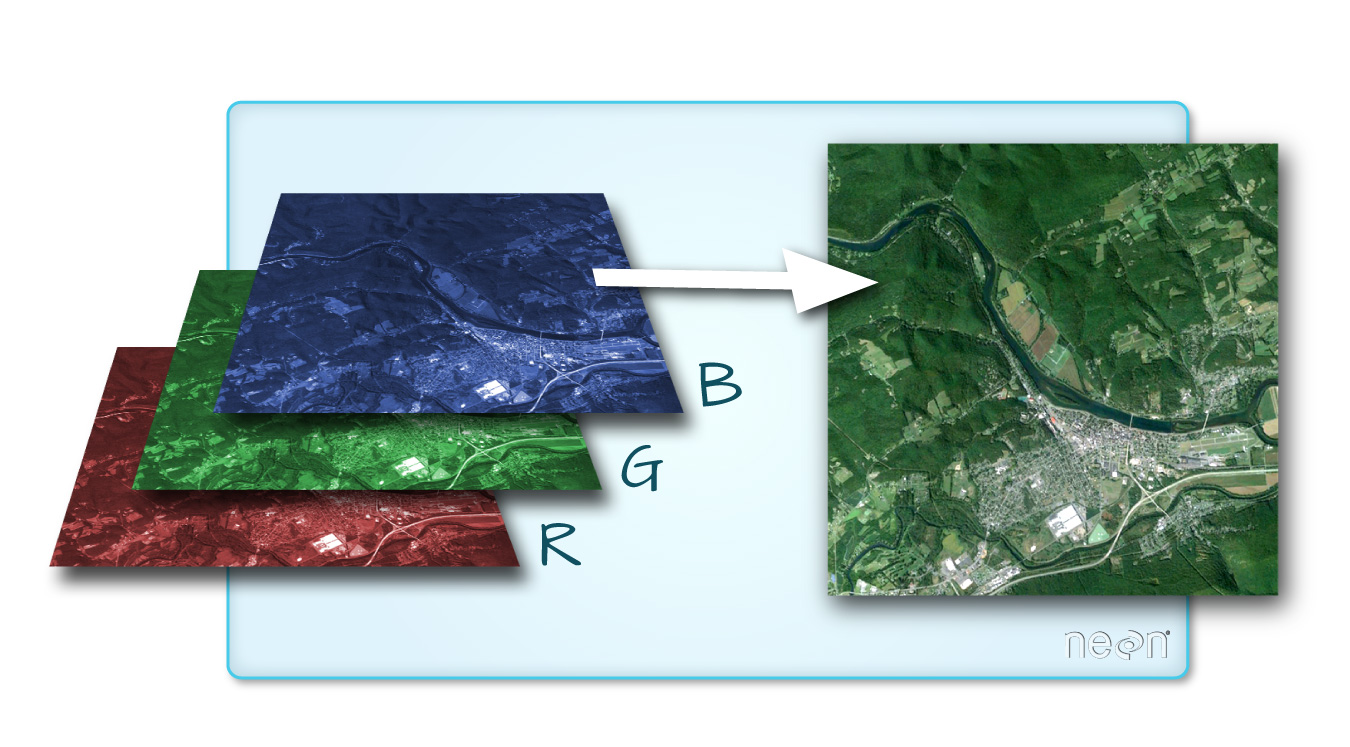
What is Multispectral Imagery?

One type of multispectral imagery that is familiar to many of us is a color image. A color image consists of three bands: red, green, and blue. Each band represents light reflected from the red, green or blue portions of the electromagnetic spectrum. The pixel brightness for each band, when composited creates the colors that you see in an image. These colors are the ones your eyes can see within the visible portion of the electromagnetic spectrum.

You can plot each band of a multi-band image individually using a grayscale color gradient. Remember from the videos that you watched in class that the LIGHTER colors represent a stronger reflection in that band. DARKER colors represent a weaker reflection.

Each Band Plotted Separately

Note there are four bands below. You are looking at the blue, green, red and near infrared bands of a NAIP image. What do you notice about the relative darkness / lightness of each image? Is one image brighter than the other?

# use stack function to read in all bands of a color image
rgb_image_3bands <- stack("data/week-07/naip/m_3910505_nw_13_1_20130926/crop/m_3910505_nw_13_1_20130926_crop.tif")
names(rgb_image_3bands) <- c("red_band", "green_band", "blue_band", "near_infrared_band")

plot(rgb_image_3bands,
     col = gray(0:100 / 100),
   box = FALSE, axes = FALSE)

You can plot the red, green and blue bands together to create an RGB image. This is what you would see with your eyes if you were in the airplane looking down at the Earth.

CIR Image

If the image has a 4th Near Infrared (NIR) band, you can create a Color Infrared (CIR, sometimes called false color) image. In a CIR image, the NIR band is plotted on the “red” band, the red band is plotted using green and the green band is plotted using blue. Thus vegetation, which reflects strongly in the NIR part of the spectrum, is colored “red.”

Other Types of Multi-Band Raster Data

Above you learned about multi-band raster data in the context of multispectral imagery. However, multi-band raster data might also contain:

1. Time series data: the same variable, over the same area, over time.
2. Multi or hyperspectral imagery: image rasters that have 4 or more (multi-spectral) or more than 10-15 (hyperspectral) bands.

About NAIP Multispectral Imagery

The multispectral imagery that you are using is collected by the National Agricultural Imagery Program (NAIP).

The National Agriculture Imagery Program (NAIP) acquires aerial imagery during the agricultural growing seasons in the continental U.S. A primary goal of the NAIP program is to make digital ortho photography available to governmental agencies and the public within a year of acquisition.

NAIP is administered by the USDA’s Farm Service Agency (FSA) through the Aerial Photography Field Office in Salt Lake City. This “leaf-on” imagery is used as a base layer for GIS programs in FSA’s County Service Centers, and is used to maintain the Common Land Unit (CLU) boundaries. – USDA NAIP Program

Read more about NAIP

NAIP is a great source of high resolution imagery across the United States. NAIP imagery is often collected with just a red, green and blue band. However, some flights include a near infrared band which is very useful for quantifying vegetation cover and health.

NAIP data access: For this lesson the USGS Earth Explorer site was used to download NAIP imagery.

Open NAIP Multispectral Imagery in R

Next, let’s explore some multispectral imagery in R. This imagery covers the site of a fire called the Cold Springs fire that occurred in Colorado near Nederland. You will learn more about this fire over the upcoming weeks.

To work with multi-band raster data you use the raster and rgdal packages. You’ll use the rgeos package to crop the data.

# load spatial packages
library(raster)
library(rgdal)
library(rgeos)

Next, open up the NAIP imagery for the Cold Springs fire study area in Colorado.

# Read in multi-band raster with raster function.
# the first band will be read in automatically
# csf = cold springs fire!
naip_csf <- raster("data/week-07/naip/m_3910505_nw_13_1_20130926/crop/m_3910505_nw_13_1_20130926_crop.tif")

# Plot band 1
plot(naip_csf,
     col = gray(0:100 / 100),
     axes = FALSE, box = FALSE,
     main = "NAIP RGB Imagery - Band 1-Red\nCold Springs Fire Scar")

# view data dimensions, CRS, resolution, attributes, and band info
naip_csf
## class      : RasterLayer 
## band       : 1  (of  4  bands)
## dimensions : 2312, 4377, 10119624  (nrow, ncol, ncell)
## resolution : 1, 1  (x, y)
## extent     : 457163, 461540, 4424640, 4426952  (xmin, xmax, ymin, ymax)
## crs        : +proj=utm +zone=13 +ellps=GRS80 +towgs84=0,0,0,0,0,0,0 +units=m +no_defs 
## source     : /root/earth-analytics/data/week-07/naip/m_3910505_nw_13_1_20130926/crop/m_3910505_nw_13_1_20130926_crop.tif 
## names      : m_3910505_nw_13_1_20130926_crop 
## values     : 0, 255  (min, max)

Notice that when you look at the attributes of RGB_Band1, you see:

band: 1 (of 4 bands)

This is R telling us that this particular raster object has more bands (4 in total). You only imported the first band.

Data Tip: The number of bands associated with a raster object can also be determined using the nbands slot. Syntax is ObjectName@file@nbands, or specifically for your file: RGB_band1@file@nbands.

Image Raster Data Values

Next, examine the raster min and max values. What is the value range?

# view min value
minValue(naip_csf)
## [1] 0

# view max value
maxValue(naip_csf)
## [1] 255

This raster contains values between 0 and 255. These values represent degrees of brightness associated with the image band. In the case of a RGB image (red, green and blue), band 1 is the red band. When you plot the red band, larger numbers (towards 255) represent pixels with more red in them (a strong red reflection). Smaller numbers (towards 0) represent pixels with less red in them (less red was reflected). To plot an RGB image, you mix red + green + blue values, using the ratio of each. The ratio of each color is determined by how much light was recorded (the reflectance value) in each band. This mixture creates one single color than in turn makes up the full color image - similar to the color image your camera phone creates.

Import a Specific Band

You use the raster() function to import specific bands in your raster object by specifying which band you want with band=N (N represents the band number you want to work with). To import the green band, you would use band = 2.

# Can specify which band you want to read in
rgb_band2 <- raster("data/week-07/naip/m_3910505_nw_13_1_20130926/crop/m_3910505_nw_13_1_20130926_crop.tif",
             band = 2)

# plot band 2
plot(rgb_band2,
     col = gray(0:100 / 100),
     axes = FALSE,
     main = "RGB Imagery - Band 2 - Green\nCold Springs Fire Scar")

# view attributes of band 2
rgb_band2
## class      : RasterLayer 
## band       : 2  (of  4  bands)
## dimensions : 2312, 4377, 10119624  (nrow, ncol, ncell)
## resolution : 1, 1  (x, y)
## extent     : 457163, 461540, 4424640, 4426952  (xmin, xmax, ymin, ymax)
## crs        : +proj=utm +zone=13 +ellps=GRS80 +towgs84=0,0,0,0,0,0,0 +units=m +no_defs 
## source     : /root/earth-analytics/data/week-07/naip/m_3910505_nw_13_1_20130926/crop/m_3910505_nw_13_1_20130926_crop.tif 
## names      : m_3910505_nw_13_1_20130926_crop 
## values     : 0, 255  (min, max)

Notice that band 2 is the second of 3 bands band: 2 (of 4 bands).

Raster Stacks in R

Above you opened and explored just one single band.Next, you will import all four image bands (red, green, blue and near-infrared) as an R RasterStack object. You will then plot a 3-band composite, or full color image.

To bring in all bands of a multi-band raster, use thestack() function. IMPORTANT: All rasters in a raster stack must have the same extent, CRS and resolution.

# Use stack function to read in all bands
naip_csf_st <-
  stack("data/week-07/naip/m_3910505_nw_13_1_20130926/crop/m_3910505_nw_13_1_20130926_crop.tif")

# view attributes of stack object
naip_csf_st
## class      : RasterStack 
## dimensions : 2312, 4377, 10119624, 4  (nrow, ncol, ncell, nlayers)
## resolution : 1, 1  (x, y)
## extent     : 457163, 461540, 4424640, 4426952  (xmin, xmax, ymin, ymax)
## crs        : +proj=utm +zone=13 +ellps=GRS80 +towgs84=0,0,0,0,0,0,0 +units=m +no_defs 
## names      : m_3910505_nw_13_1_20130926_crop.1, m_3910505_nw_13_1_20130926_crop.2, m_3910505_nw_13_1_20130926_crop.3, m_3910505_nw_13_1_20130926_crop.4 
## min values :                                 0,                                 0,                                 0,                                 0 
## max values :                               255,                               255,                               255,                               255

inMemory(naip_csf_st)
## [1] FALSE

The stack is a good start to working with all the bands. However, if you want to plot and process the data, a rasterbrick is faster. Next, convert the stack to a brick.

A rasterbrick in R, saves all of the bands in the same place making it faster when you process the data.

# convert data to raster brick
naip_csf_br <- brick(naip_csf_st)
inMemory(naip_csf_br)
## [1] FALSE

You can view the attributes of each band the stack using naip_csf_br@layers. Or if you have hundreds of bands, you can specify which band you’d like to view attributes for using an index value: naip_csf_br[[1]]. You can also use the plot() and hist() functions on the RasterStack to plot and view the distribution of raster band values.

# view raster attributes
naip_csf_br
## class      : RasterBrick 
## dimensions : 2312, 4377, 10119624, 4  (nrow, ncol, ncell, nlayers)
## resolution : 1, 1  (x, y)
## extent     : 457163, 461540, 4424640, 4426952  (xmin, xmax, ymin, ymax)
## crs        : +proj=utm +zone=13 +ellps=GRS80 +towgs84=0,0,0,0,0,0,0 +units=m +no_defs 
## source     : /tmp/RtmpzcDiNN/raster/r_tmp_2019-09-03_191435_109_75703.grd 
## names      : m_3910505_nw_13_1_20130926_crop.1, m_3910505_nw_13_1_20130926_crop.2, m_3910505_nw_13_1_20130926_crop.3, m_3910505_nw_13_1_20130926_crop.4 
## min values :                                 0,                                 0,                                 0,                                 0 
## max values :                               255,                               255,                               255,                               255

View attributes of one band.

# view attributes for one band
naip_csf_br[[1]]
## class      : RasterLayer 
## band       : 1  (of  4  bands)
## dimensions : 2312, 4377, 10119624  (nrow, ncol, ncell)
## resolution : 1, 1  (x, y)
## extent     : 457163, 461540, 4424640, 4426952  (xmin, xmax, ymin, ymax)
## crs        : +proj=utm +zone=13 +ellps=GRS80 +towgs84=0,0,0,0,0,0,0 +units=m +no_defs 
## source     : /tmp/RtmpzcDiNN/raster/r_tmp_2019-09-03_191435_109_75703.grd 
## names      : m_3910505_nw_13_1_20130926_crop.1 
## values     : 0, 255  (min, max)

You can view a histogram of each band in your stack. This is useful to better understand the distribution of reflectance values for each band.

# view histogram for each band
hist(naip_csf_br,
     maxpixels = ncell(naip_csf_br),
     col = "purple")

Plot each band individually.

# plot 4 bands separately
plot(naip_csf_br,
     col = gray(0:100 / 100))

You can plot just one band too.

# plot band 2
plot(naip_csf_br[[2]],
     main = "NAIP Band 2\n Coldsprings Fire Site",
     col = gray(0:100 / 100))

RGB Data

Previously you’ve explored the single bands in your rasterstack. Next, you’ll plot an RGB image.

Use plotRGB() to Create a Composite 3 Band Image

To render a 3 band, color image in R, you use plotRGB().

This function allows us to:

1. Identify what bands you want to render in the red, green and blue regions. The plotRGB() function defaults to a 1 = red, 2 = green, and 3 = blue band order. However, you can define what bands you’d like to plot manually. Manual definition of bands is useful if you have, for example a near-infrared band and want to create a color infrared image.
2. Adjust the stretch of the image to increase or decrease contrast.

Let’s plot your 3-band image.

# Create an RGB image from the raster stack
plotRGB(naip_csf_br,
        r = 1, g = 2, b = 3,
        main = "RGB image \nColdsprings fire scar")

To add a title to your plot, adjust the parameters as follows:

• col.axis = "white": set the axes to render in white. if you turn off the axes then the plot title will also be turned off.
• col.lab = "white": turn plot tick mark labels to white.
• tck = 0: turn off plot “ticks.”

Finally after the plot code if you set box(col = "white") it removes the line that is drawn alongside of your plot.

# adjust the plot parameters to render the axes using white
# this is a way to "trick" R
par(col.axis = "white", col.lab = "white", tck = 0)
plotRGB(naip_csf_br,
        r = 1, g = 2, b = 3,
        axes = TRUE,
        main = "NAIP RGB image \nColdsprings fire scar")
box(col = "white") # turn all of the lines to white

Apply a Stretch to Normalize the Colors in the Image

The image above looks pretty good. You can explore whether applying a stretch to the image might improve clarity and contrast using stretch="lin" or stretch = "hist".

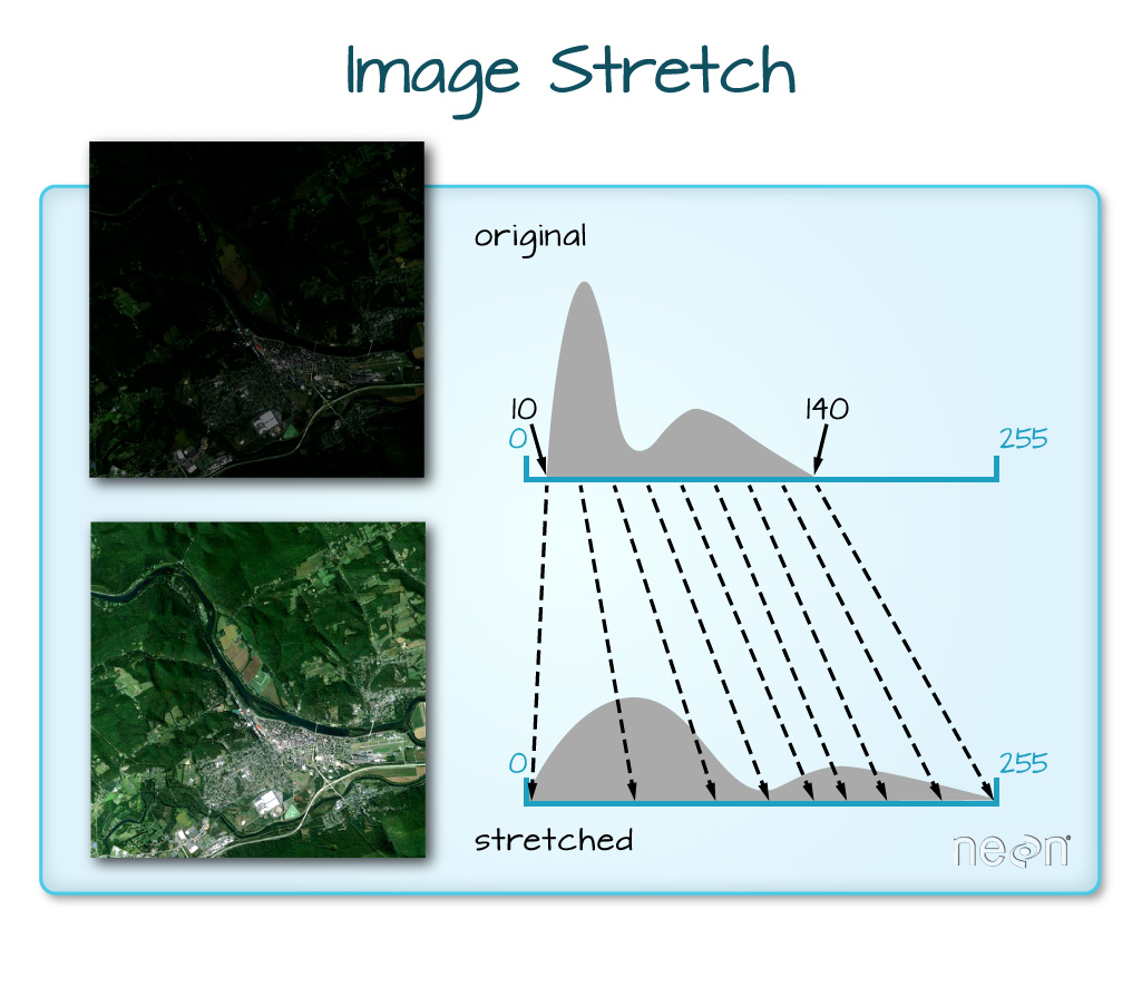
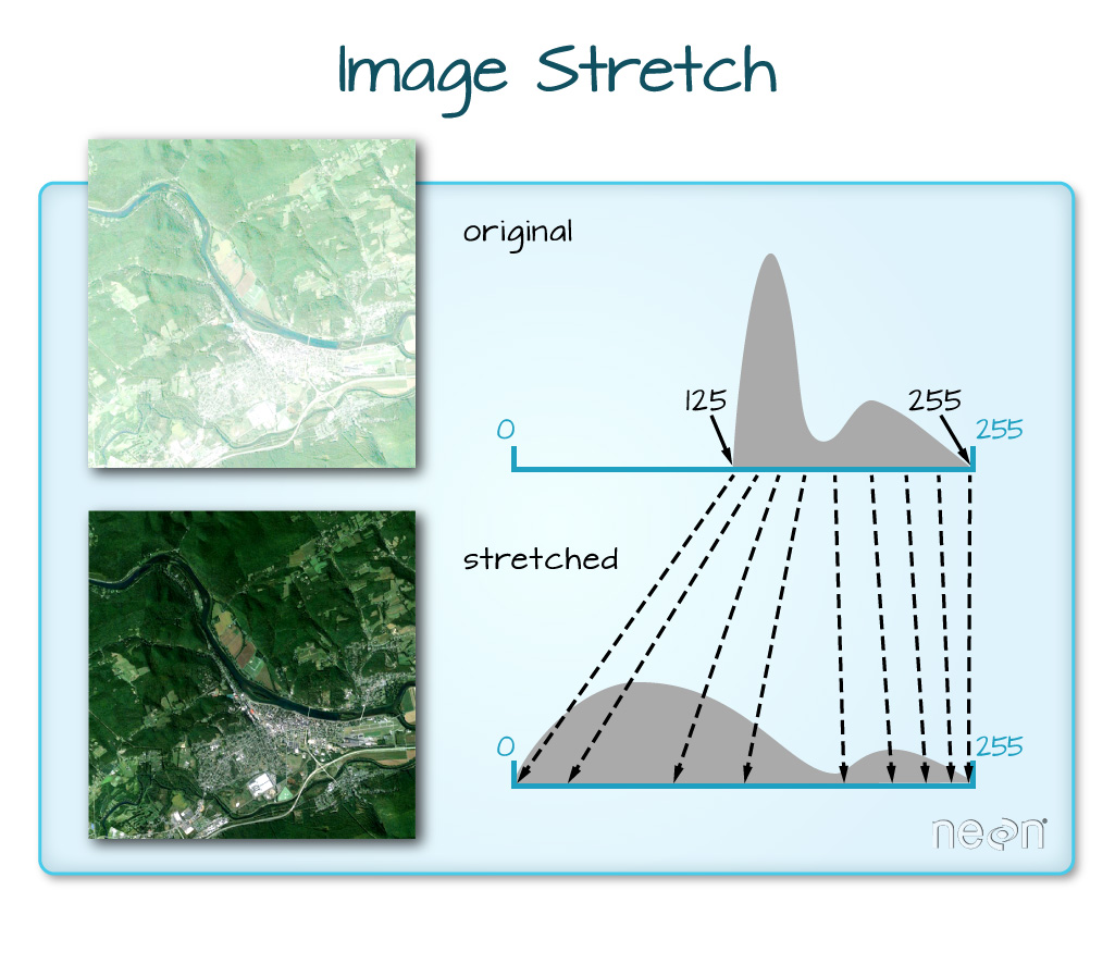
# what does stretch do?
par(col.axis = "white", col.lab = "white", tck = 0)
plotRGB(naip_csf_br,
        r = 1, g = 2, b = 3,
        axes = TRUE,
        stretch = "lin",
        main = "NAIP RGB plot with linear stretch\nColdsprings fire scar")

What does the image look like using a different stretch? Any better? Worse?

par(col.axis = "white", col.lab = "white", tck = 0)
plotRGB(naip_csf_br,
        r = 1, g = 2, b = 3,
        axes = TRUE,
        scale = 800,
        stretch = "hist",
        main = "NAIP RGB plot with hist stretch\nColdsprings fire scar")
box(col = "white") # turn all of the lines to white

In this case, the stretch doesn’t enhance the contrast of your image significantly given the distribution of reflectance (or brightness) values is distributed well between 0 and 255. You are lucky! Your NAIP imagery has been processed well and thus you don’t need to worry about image stretch.

More on RasterStacks vs RasterBricks in R

The R RasterStack and RasterBrick object types can both store multiple bands. However, how they store each band is different. The bands in a RasterStack are stored as links to raster data that is located somewhere on your computer. A RasterBrick contains all of the objects stored within the actual R object. In most cases, you can work with a RasterBrick in the same way you might work with a RasterStack. However a RasterBrick is often more efficient and faster to process - which is important when working with larger files.

• More on Raster Bricks

You can turn a RasterStack into a RasterBrick in R by using brick(StackName). Let’s use the object.size() function to compare stack and brick R objects.

# view size of the RGB_stack object that contains your 3 band image
object.size(naip_csf_st)
## 56888 bytes

# convert stack to a brick
naip_brick_csf <- brick(naip_csf_st)

# view size of the brick
object.size(naip_brick_csf)
## 161927968 bytes

Notice that in the RasterBrick, all of the bands are stored within the actual object. Thus, the RasterBrick object size is much larger than the RasterStack object.

You use plotRGB to block a RasterBrick too.

par(col.axis = "white", col.lab = "white", tck = 0)
# plot brick
plotRGB(naip_brick_csf,
  main = "NAIP plot from a rasterbrick",
  axes = TRUE)
box(col = "white") # turn all of the lines to white