Lesson 2. Extract Raster Values Using Vector Boundaries in R
Learning Objectives
After completing this tutorial, you will be able to:
- Use the
extract()function to extract raster values using a vector extent or set of extents. - Create a scatter plot with a one-to-one line in
R. - Understand the concept of uncertainty as it’s associated with remote sensing data.
What You Need
You will need a computer with internet access to complete this lesson and the data for week 4 of the course.
# load libraries
library(raster)
library(rgdal)
library(rgeos)
library(ggplot2)
library(dplyr)

options(stringsAsFactors = FALSE)

# set working directory
# setwd("path-here/earth-analytics")
Import Canopy Height Model
First, you will import a canopy height model created by the NEON project. In the
previous lessons / weeks you learned how to make a canopy height model by
subtracting the digital elevation model (DEM) from the digital surface model (DSM).
# import canopy height model (CHM).
SJER_chm <- raster("data/week-04/california/SJER/2013/lidar/SJER_lidarCHM.tif")
SJER_chm
## class      : RasterLayer
## dimensions : 5059, 4296, 21733464  (nrow, ncol, ncell)
## resolution : 1, 1  (x, y)
## extent     : 254571, 258867, 4107303, 4112362  (xmin, xmax, ymin, ymax)
## crs        : +proj=utm +zone=11 +datum=WGS84 +units=m +no_defs +ellps=WGS84 +towgs84=0,0,0
## source     : /root/earth-analytics/data/week-04/california/SJER/2013/lidar/SJER_lidarCHM.tif
## names      : SJER_lidarCHM
## values     : 0, 45.88  (min, max)

# view distribution of pixel values
hist(SJER_chm,
     main = "Histogram of Canopy Height\n NEON SJER Field Site",
     col = "springgreen",
     xlab = "Height (m)")

There are a lot of values in your CHM that == 0. Let’s set those to NA and plot
again.
# set values of 0 to NA as these are not trees
SJER_chm[SJER_chm == 0] <- NA

# plot the modified data
hist(SJER_chm,
     main = "Histogram of Canopy Height\n pixels==0 set to NA",
     col = "springgreen",
     xlab = "Height (m)")

Part 2. Does Your CHM Data Compare to Field Measured Tree Heights?
You now have a canopy height model for your study area in California. However, how
do the height values extracted from the CHM compare to your laboriously collected,
field measured canopy height data? To figure this out, you will use in situ collected
tree height data, measured within circular plots across your study area. You will compare
the maximum measured tree height value to the maximum lidar derived height value
for each circular plot using regression.
For this activity, you will use the a csv (comma separate value) file,
located in SJER/2013/insitu/veg_structure/D17_2013_SJER_vegStr.csv.
# import plot centroids
SJER_plots <- readOGR("data/week-04/california/SJER/vector_data/SJER_plot_centroids.shp")
## OGR data source with driver: ESRI Shapefile
## Source: "/root/earth-analytics/data/week-04/california/SJER/vector_data/SJER_plot_centroids.shp", layer: "SJER_plot_centroids"
## with 18 features
## It has 5 fields

# Overlay the centroid points and the stem locations on the CHM plot
plot(SJER_chm,
     main = "SJER Plot Locations",
     col = gray.colors(100, start = .3, end = .9))

# pch 0 = square
plot(SJER_plots,
     pch = 16,
     cex = 2,
     col = 2,
     add = TRUE)

Extract CMH Data Within 20m Radius of Each Plot Centroid
Next, you will create a boundary region (called a buffer) representing the spatial
extent of each plot (where trees were measured). You will then extract all CHM pixels
that fall within the plot boundary to use to estimate tree height for that plot.
There are a few ways to go about this task. If your plots are circular, then you can
use the extract() function.
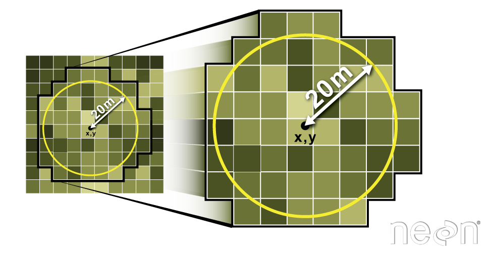
Extract Plot Data Using Circle: 20m Radius Plots
# Insitu sampling took place within 40m x 40m square plots, so you use a 20m radius.
# Note that below will return a data.frame containing the max height
# calculated from all pixels in the buffer for each plot
SJER_height <- raster::extract(SJER_chm,
                    SJER_plots,
                    buffer = 20, # specify a 20 m radius
                    fun = mean, # extract the MEAN value from each plot
                    sp = TRUE, # create spatial object
                    stringsAsFactors = FALSE)

# view structure of the spatial data frame attribute table
head(SJER_height@data)
##    Plot_ID  Point northing  easting plot_type SJER_lidarCHM
## 1 SJER1068 center  4111568 255852.4     trees     11.544348
## 2  SJER112 center  4111299 257407.0     trees     10.355685
## 3  SJER116 center  4110820 256838.8     grass      7.511956
## 4  SJER117 center  4108752 256176.9     trees      7.675347
## 5  SJER120 center  4110476 255968.4     grass      4.591176
## 6  SJER128 center  4111389 257078.9     trees      8.979005
# note that this is a spatial points data frame
class(SJER_height)
## [1] "SpatialPointsDataFrame"
## attr(,"package")
## [1] "sp"
Looking at your new spatial points data frame, you can see a field named SJER_lidarCHM. This is the column name of the mean height for each plot location. Let’s rename that to be something more meaningful.
# raname
colnames(SJER_height@data)[6]
## [1] "SJER_lidarCHM"

# rename the column
colnames(SJER_height@data)[6] <- "lidar_mean_ht"
head(SJER_height@data)
##    Plot_ID  Point northing  easting plot_type lidar_mean_ht
## 1 SJER1068 center  4111568 255852.4     trees     11.544348
## 2  SJER112 center  4111299 257407.0     trees     10.355685
## 3  SJER116 center  4110820 256838.8     grass      7.511956
## 4  SJER117 center  4108752 256176.9     trees      7.675347
## 5  SJER120 center  4110476 255968.4     grass      4.591176
## 6  SJER128 center  4111389 257078.9     trees      8.979005
Explore the Data Distribution
If you want to explore the data distribution of pixel height values in each plot,
you could remove the fun call to max and generate a list.
cent_ovrList <- extract(chm,centroid_sp,buffer = 20). It’s good to look at the
distribution of values you’ve extracted for each plot. Then you could generate a
histogram for each plot hist(cent_ovrList[[2]]). If you wanted, you could loop
through several plots and create histograms using a for loop.
# cent_ovrList <- extract(chm,centroid_sp,buffer = 20)
# create histograms for the first 5 plots of data
# for (i in 1:5) {
#  hist(cent_ovrList[[i]], main=(paste("plot",i)))
#  }
Plot by Height
# plot canopy height model
plot(SJER_chm,
     main = "Vegetation Plots \nSymbol size by Average Tree Height",
     legend = FALSE)

# add plot location sized by tree height
plot(SJER_height,
     pch = 19,
     cex = (SJER_height$lidar_mean_ht)/10, # size symbols according to tree height attribute normalized by 10
     add = TRUE)

# place legend outside of the plot
par(xpd = TRUE)
legend(SJER_chm@extent@xmax + 250,
       SJER_chm@extent@ymax,
       legend = "plot location \nsized by \ntree height",
       pch = 19,
       bty = 'n')

Share on
Twitter Facebook Google+ LinkedIn
Leave a Comment