Lesson 4. Homework Challenge: Plot USGS Stream Discharge Data in R
In this data lesson, you explore and visualize stream discharge time series data collected by the United States Geological Survey (USGS). You will use everything that you learned in the previous lessons to create your plots. You will use these plots in the report that you submit for your homework.
Note: this page just shows you what the plots should look like. You will need to use your programming skills to create the plots!
Learning Objectives
After completing this tutorial, you will be able to:
- Plot USGS Stream Discharge time series data in
R
What You Need
You need R and RStudio to complete this tutorial. Also you should have
an earth-analytics directory set up on your computer with a /data
directory with it.
R Libraries to Install:
- ggplot2:
install.packages("ggplot2") - dplyr:
install.packages("dplyr")
If you haven’t already downloaded this data (from the previous lesson), do so now.
About the Data - USGS Stream Discharge Data
The USGS has a distributed network of aquatic sensors located in streams across the United States. This network monitors a suit of variables that are important to stream morphology and health. One of the metrics that this sensor network monitors is Stream Discharge, a metric which quantifies the volume of water moving down a stream. Discharge is an ideal metric to quantify flow, which increases significantly during a flood event.
As defined by USGS: Discharge is the volume of water moving down a stream or river per unit of time, commonly expressed in cubic feet per second or gallons per day. In general, river discharge is computed by multiplying the area of water in a channel cross section by the average velocity of the water in that cross section.

As you can imagine, stream gages can be sensitive to high flows and in the case of an extreme event like a flood are sometimes damaged. However, during the 2013 floods, one stream gage in Boulder, Colorado remained in tact. USGS stream gauge 06730200 located on Boulder Creek at North 75th St. collected data that you will use in the lesson below!
Work with USGS Stream Gage Data
Let’s begin by loading your libraries and setting your working directory.
# set your working directory
# setwd("working-dir-path-here")

# load packages
library(ggplot2) # create efficient, professional plots
library(dplyr) # data manipulation

# set strings as factors to false
options(stringsAsFactors = FALSE)
Import USGS Stream Discharge Data into R
Let’s first import your data using the read.csv() function.
discharge <- read.csv("data/week-02/discharge/06730200-discharge-daily-1986-2013.csv",
                      header = TRUE)

# view first 6 lines of data
head(discharge)
##   agency_cd site_no datetime disValue qualCode
## 1      USGS 6730200  10/1/86       30        A
## 2      USGS 6730200  10/2/86       30        A
## 3      USGS 6730200  10/3/86       30        A
## 4      USGS 6730200  10/4/86       30        A
## 5      USGS 6730200  10/5/86       30        A
## 6      USGS 6730200  10/6/86       30        A
Challenge
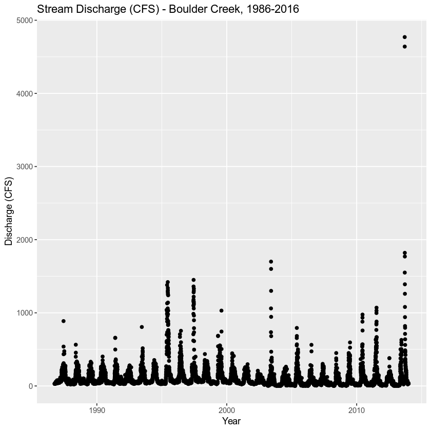
Now that the data are imported, plot disValue (discharge value) over time.
To do this, you will need to use everything that you learned in the previous lessons.
Hint: when converting the date, take a close look at the format of the date -
is the year 4 digits (including the century) or just 2? Use ?strptime to figure
out what format elements you’ll need to include to get the date right.
Your plot should look something like the one below:

Challenge
Similar to the previous lesson, take the cleaned discharge data that you just
plotted and subset it to the time span
of 2013-08-15 to 2013-10-15. Use dplyr pipes and the filter() function
to perform the subset.
Plot the data with ggplot(). Your plot should look like the one below.

Additional Resources
Additional information on USGS streamflow measurements and data:
- Find peak streamflow for other locations
- USGS: How streamflow is measured
- USGS: How streamflow is measured, Part II
- USGS National Streamflow Information Program Fact Sheet
API Data Access
USGS data can be downloaded via an API using a command line interface. This is particularly useful if you want to request data from multiple sites or build the data request into a script. Read more here about API downloads of USGS data.
Share on
Twitter Facebook Google+ LinkedIn
Leave a Comment